Why Does Biological Evolution Work?

Original article: https://writings.stephenwolfram.com/2024/05/why-does-biological-evolution-work-a-minimal-model-for-biological-evolution-and-other-adaptive-processes/

A model of life

Why does biological evolution work? Why does machine learning work? Both are adaptive processes whose results surprise us. What is happening? Here I will concentrate on biological evolution, although much of the discussion also applies to machine learning—a subject I plan to discuss in more detail elsewhere.

What is the simplest biologically plausible model? My central idea is to view organisms as computational systems that develop by following simple underlying rules. Those rules effectively constitute the organism’s genotype; running them produces its phenotype. Cellular automata provide simple examples. Here is one with three possible cell colors, with its rule on the left and the behavior it generates on the right:

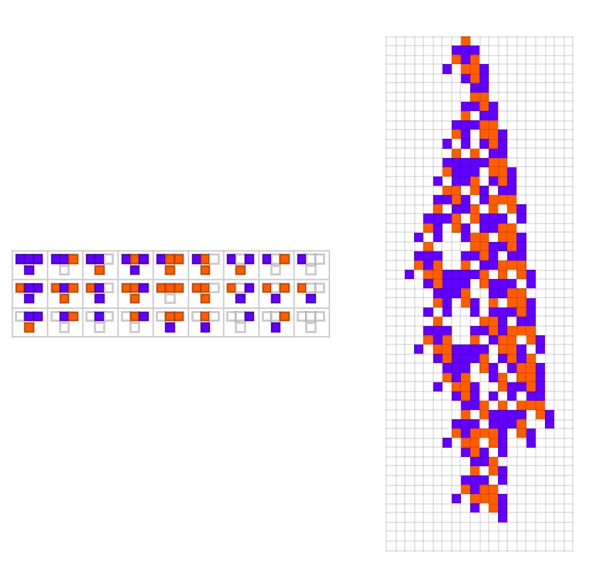
Starting from a single cell—the red square—we see a structure grow from this seed, then disappear after 51 steps. In a sense, it is already remarkable to obtain a structure that neither lasts forever nor vanishes immediately, but survives for exactly 51 steps in this example.

Suppose, however, that we begin with a simple null rule under which every pattern immediately disappears. Could adaptive evolution eventually produce the rule above? Imagine a series of randomly chosen point mutations, each changing one outcome in the rule:

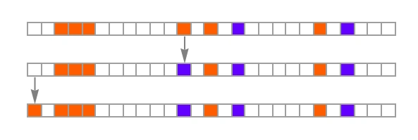
At each step, in a minimal analogue of natural selection, accept a mutation if it extends the lifetime without making it infinite, or at least leaves it unchanged. Reject mutations that shorten the lifetime or make it infinite. This process can indeed adaptively evolve the rule above. Here we show only the intermediate points at which lifetime increases:

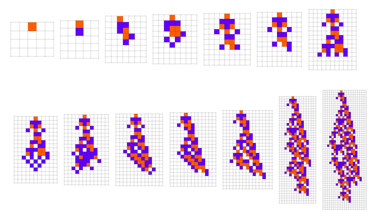
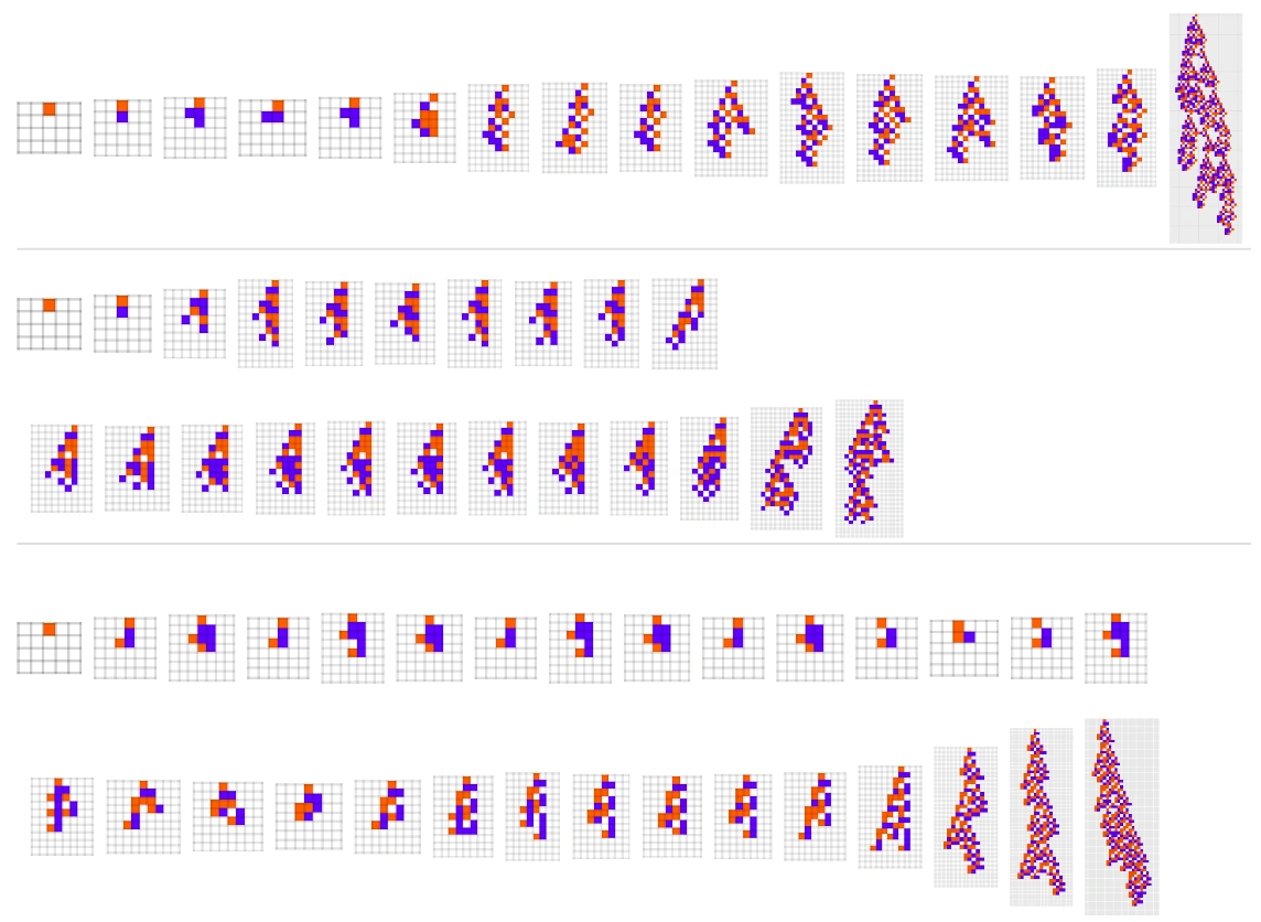
Different random mutation sequences produce different rule sequences. Remarkably, though, progress is possible in almost every case, often reaching rules that generate long-lived patterns—here with lifetimes of 107, 162, and 723 steps—and complex morphological structures:

[Image unavailable: the source image is missing.]

Is it obvious that this simple adaptive process should be able to steer things toward such results? No. Yet its ability to do so seems central to why biological evolution works.

Looking at these sequences, we often see different mechanisms emerge in different rule sequences to produce long lifetimes. Typically, a simple version of a mechanism appears first, then develops, becomes elaborated, and is built upon as adaptation continues—reminiscent of what we often see in the fossil record.

Let us look more closely at our simple model. For the three-color, nearest-neighbor cellular automata considered here ($k=3, r=1$), there are 26 relevant rule cases ($3^3-1$), or 27 if we do not impose the background condition. A point mutation changes a single case to one of two alternative outcomes ($3-1$), giving a total of 52 possible point mutations ($26\times2$) for a given rule.

Starting with this rule:

the possible single-point mutations are:

Even these point mutations produce a considerable variety of behavior:

[Image unavailable: the source image is missing.]

In many cases, the generated pattern is exactly the same as that of the original rule. Other patterns die out sooner—or never die out, either becoming periodic or growing indefinitely. In this particular example, only one mutation achieves higher fitness by extending the lifetime.

In a sequence of random mutations, many will produce shorter-lived patterns or indefinitely surviving, “tumorous” ones. We discard these—or, in biological language, they are selected against:

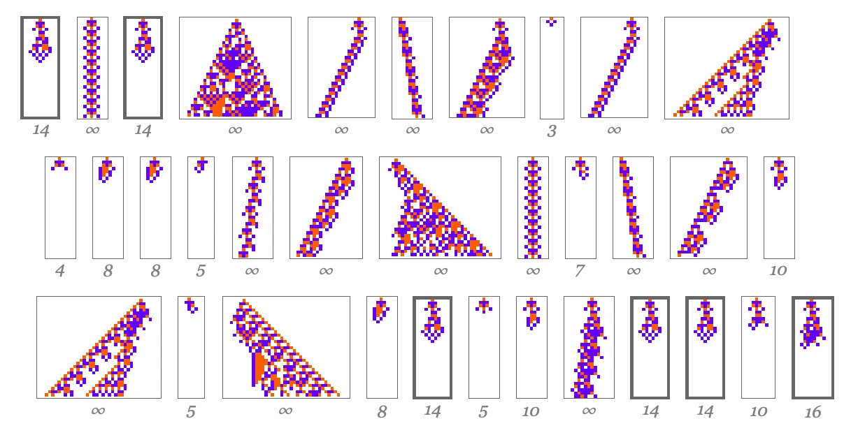
Many neutral mutations remain, however, leaving the final pattern unchanged, or at least producing one of the same lifetime. At first they may seem ineffective. In fact, they are crucial: they allow point mutations to accumulate into larger changes that can eventually produce longer-lived patterns.

[Image unavailable: the source image is missing.]

For the adaptive process above, the total numbers of point mutations between successive fitness milestones—each representing a longer lifetime—are:

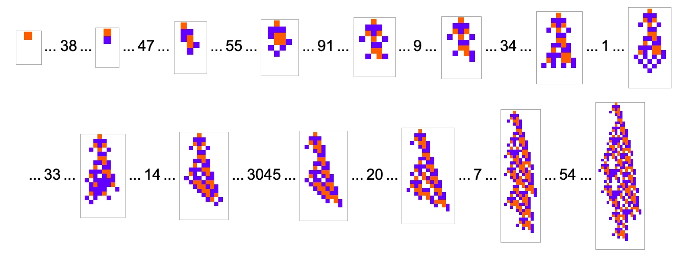
Here are the underlying rules at those milestones. The numbers count retained mutations, excluding mutations that merely go back and forth:

[Image unavailable: the source image is missing.]

Another perspective is to take the full sequence of accepted rules and plot it in a dimensionally reduced rendering of the 27-dimensional rule space:

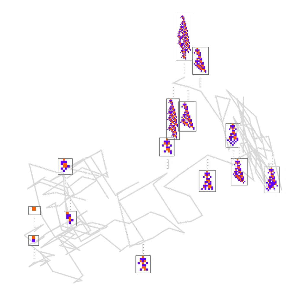
Some phases involve extensive wandering and require many mutations before progress occurs. Others move much faster and require fewer mutations.

We can also plot the greatest lifetime reached against the total number of mutations:

[Image unavailable: the source image is missing.]

There are plateaus, including a very long one, during which no progress occurs. Occasionally these are interrupted by substantial sudden changes, often caused by a single mutation.

Including rejected mutations reveals considerable activity even on a plateau. The activity simply fails to make progress. Each red point below the plateau represents an unsuccessful mutation, or an organism that did not survive selection:

[Image unavailable: the source image is missing.]

Notably, a plateau can contain multiple different phenotypic patterns. Here is what happens in this example:

[Image unavailable: the source image is missing.]

Even within these phenotypically different cases, many genotypically different rules may exist. This is not entirely surprising: typically only part of a rule is coding. Other parts are noncoding, never sampled while the pattern develops.

Here, for example, we highlight the cells at each fitness milestone that use fresh, previously unsampled rule cases:

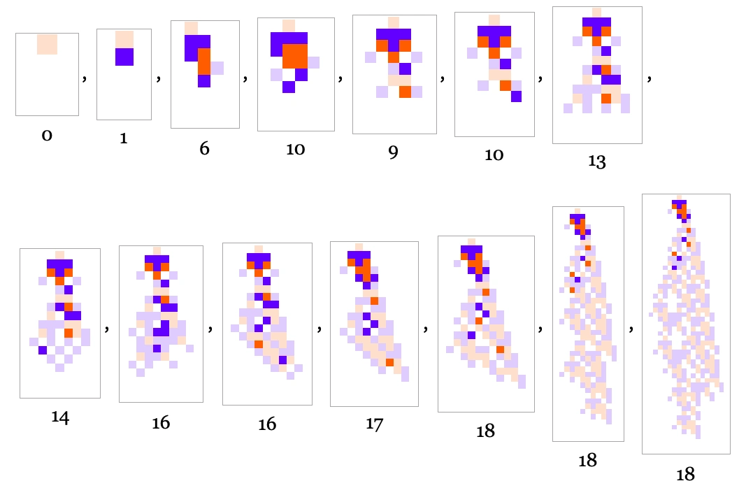
Even in the final rule shown, only 18 of the 26 relevant cases are sampled when the pattern grows from the specified single-red-cell initial condition. Eight cases are therefore undetermined by the phenotype, suggesting that $3^8=6561$ genotypes—or rules—could produce the same outcome.

So far, we have focused on one random mutation sequence. What if we consider many? Here are the increases in maximum lifetime, or fitness, for 100 different sequences:

[Image unavailable: the source image is missing.]

Perhaps the most striking observation is that these adaptive processes do not seem to become permanently stuck. Progress may take time, producing long plateaus, but the plots suggest that adaptive evolution eventually finds a way. As the lifetime distribution develops, rules tend to generate longer-lived patterns:

[Image unavailable: the source image is missing.]

The multiway graph of all possible mutation histories

So far we have discussed paths through adaptive evolution determined by particular random mutation sequences. To understand the process more fully, however, we can use a more powerful approach: following ideas from our Physics Project, the ruliad, and related work, study the multiway graph of all possible paths rather than individual histories. In biological terms, this also lets us discuss the adaptive evolution of populations rather than only individual sequences of organisms.

Let us start afresh, replacing the three-color cellular automata of the previous section with two-color, nearest-neighbor cellular automata. There are only 128 relevant rules. How are they related by point mutations? We can construct a graph showing every way a rule in this set can become another through a single mutation:

[Image unavailable: the source image is missing.]

If we consider five-bit rather than seven-bit rules, only 16 relevant rules remain, and the possible-mutation graph clearly has the form of a Boolean hypercube:

[Image unavailable: the source image is missing.]

Suppose we start with the null rule [Image unavailable: the source image is missing.]. Enumerate the rules obtainable by one point mutation—the rules directly connected to it in the graph—and examine their behavior from an initial condition such as :

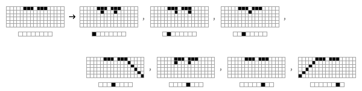
Some count as progress because they produce longer-lived patterns, although the increase is small, from one step to two. Others make no progress or produce patterns that last forever. Retaining only mutations that do not shorten the lifetime or make it infinite gives a multiway graph of all possible mutation paths:

[Image unavailable: the source image is missing.]

Although this graph contains only 15 rules, it already hints at important phenomena. Fitness-neutral mutations can happen in either direction. Many other mutations are one-way, because reversing them would reduce fitness. A notable feature is that once a path commits to one part of the graph, other parts may become inaccessible—suggesting an analogy with branches of the tree of life.

Beyond two-color, nearest-neighbor ($k=2,r=1$) automata, consider $k=2,r=\frac{3}{2}$. Here is a typical example:

For $k=2,r=1$ there are 128 relevant rules, or $2^{2^3-1}$. For $k=2,r=\frac{3}{2}$ there are 32,768, or $2^{2^4-1}$. Starting again from the null rule with the same initial condition, here are examples of adaptive evolutionary paths:

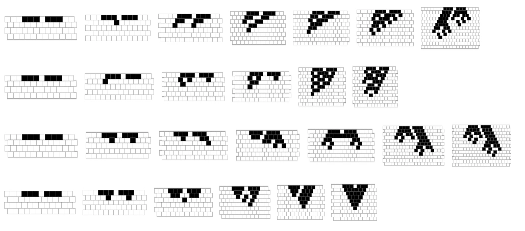
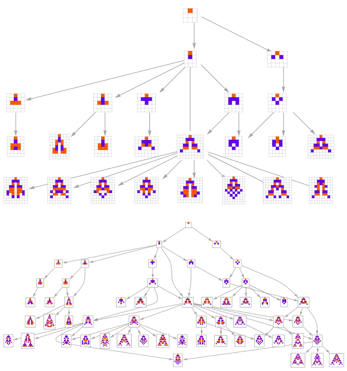
Here is the beginning of the corresponding multiway graph, showing rules reachable in at most two mutations from the null rule:

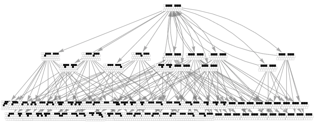
The graph contains many fitness-neutral sets: collections of rules with the same fitness that mutations can interconvert. Some examples are:

[Image unavailable: the source image is missing.]

In the first example, every genotypic rule in the neutral set generates the same phenotypic morphology. Other neutral sets contain several morphologies.

Including every individual rule gives a full $k=2,r=\frac{3}{2}$ multiway graph with 1,884 nodes. Choosing a single representative rule from each neutral set gives a more manageable graph with 86 nodes:

[Image unavailable: the source image is missing.]

Keeping only one representative from pairs of patterns related by left–right symmetry further reduces the graph to 49 nodes:

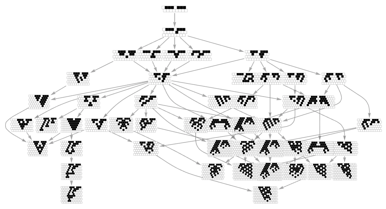
There is considerable structure, including branching and merging paths. Overall, however, different parts separate into distinct branches in which adaptive evolution explores different ways to improve fitness—that is, pattern lifetime.

Fitness-neutral sets can be viewed as equivalence classes of rules. Their structure varies: a set might contain only one member, many members but few morphologies, or a distinct morphology for every member:

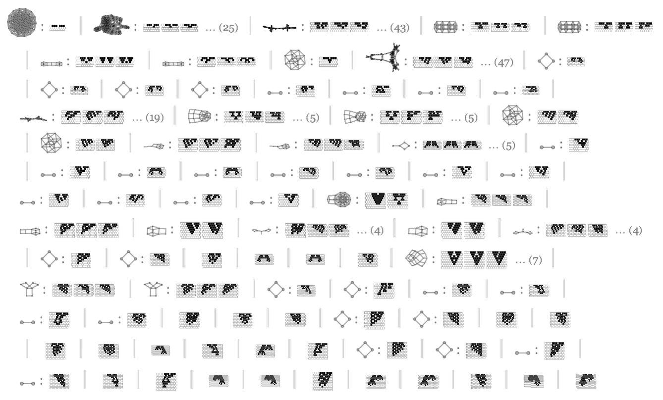
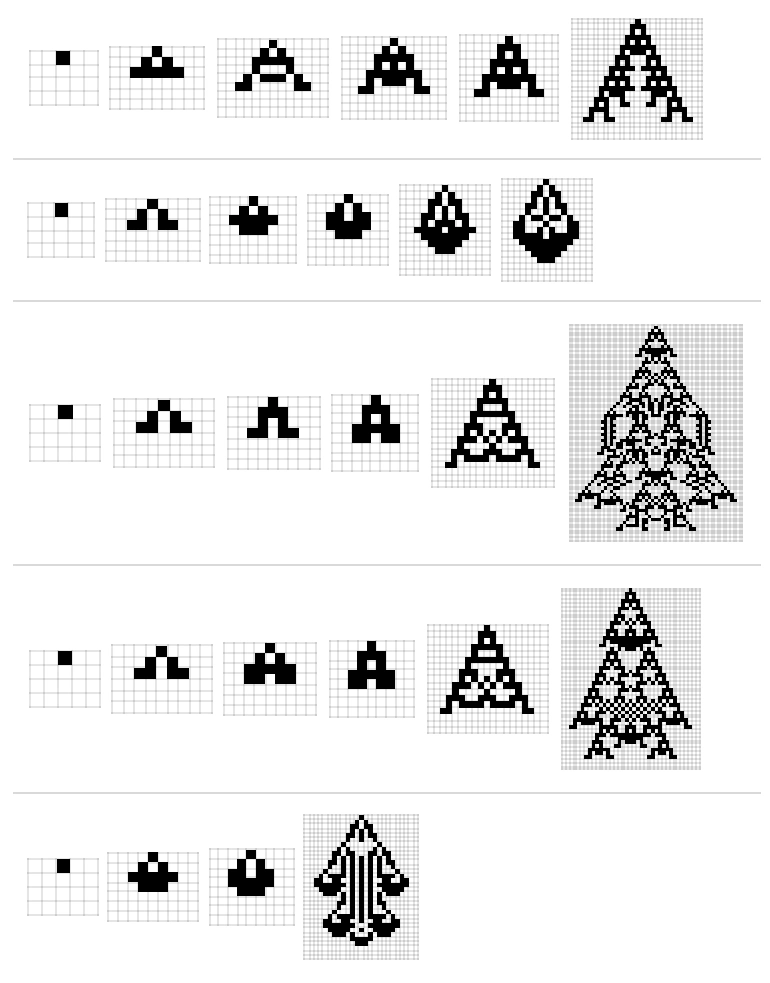
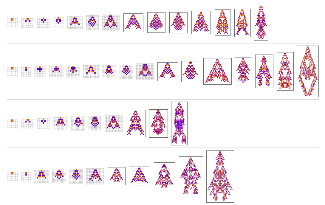
What about larger rule spaces? For $k=2,r=2$, there are roughly two billion relevant rules, or $2^{2^5-1}$. Restricting to left–right-symmetric rules reduces the count to 524,288. Here are adaptive rule sequences that start at the null rule, permit only symmetry-preserving mutations, and use a single black cell as their initial condition:

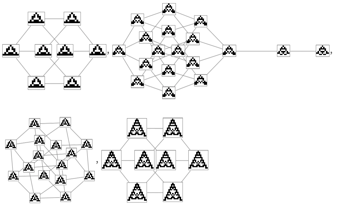
Again we can identify neutral sets. This time, in the great majority of cases, all members of a set generate the same pattern:

After collapsing neutral sets, we can compute the complete, transitively reduced multiway graph of symmetric $k=2,r=2$ rules. It has 60 nodes:

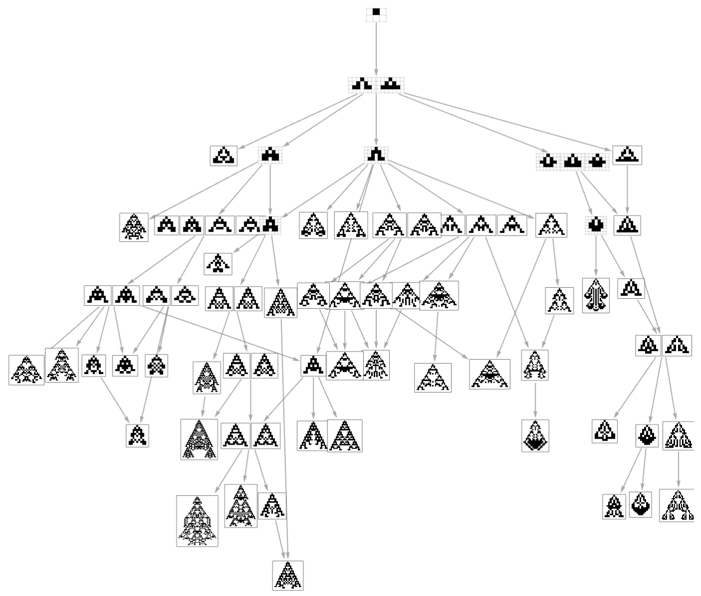
In this reduced graph, every edge represents a mutation that improves fitness. An actual path based on random mutations, however, can wander back and forth within a neutral set arbitrarily many times—not to mention trying mutations that reduce fitness—before reaching an improving mutation. Thus, although the reduced graph requires at most nine steps to reach any rule from the null rule, an actual adaptive history may take arbitrarily many steps because of neutral wandering.

Here is the sequence of accepted mutations in one particular process. Improving mutations are highlighted, with numbers recording rejected mutations:

[Image unavailable: the source image is missing.]

We can see the back-and-forth movement within neutral sets, cycling through morphologies. This is one route to the final pattern; other routes may involve fewer mutations.

Indeed, the graph gives an absolutely shortest path:

[Image unavailable: the source image is missing.]

Its sequence of rules is:

[Image unavailable: the source image is missing.]

We begin at the null rule, making one point mutation at each step, although symmetry sometimes requires changing two bits together. The first few mutations leave phenotypic behavior unchanged. After six mutations have accumulated, a morphologically different behavior appears. Just three additional mutations produce the final pattern.

The earlier random sequence reached the same outcome by a much more winding route, with 169 mutations, many canceling one another:

[Image unavailable: the source image is missing.]

The multiway graph defines which evolutionary paths are possible. What about their probabilities? If each point mutation is equally likely, we can analyze flow through the graph to determine the probability of eventually reaching each rule. Redder colors here indicate greater probability:

[Image unavailable: the source image is missing.]

The fitness landscape

The multiway graph gives a global view of adaptive evolution. Local details, however, are often more useful for understanding how the process unfolds. Imagine all possible rules arranged in a space, with adaptive evolution finding paths through it. We can also imagine a fitness landscape defined on that space, and evolution following a path upward toward peaks of greater fitness.

Return to our first example, adaptive evolution in the space of three-color cellular automata. At every step there are 52 possible point mutations. Each represents a step in a different direction in the 26-dimensional rule space.

Here is a visualization for the particular evolutionary path in that example:

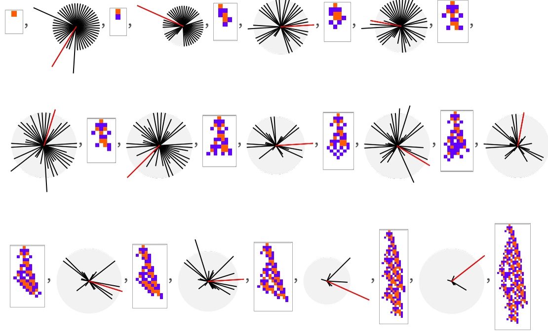
What we show is a sequence of decisions between successive fitness milestones. Radial directions represent possible mutations, and line lengths are proportional to the fitness each mutation would produce. At every step, a gray disk represents the previous fitness. Many mutations lead to lower fitness and lie inside the disk. At least some lead to greater fitness and escape it.

A multiway graph follows every mutation that improves fitness. For the particular path discussed here, however, we assume one is chosen randomly from this set at each step, indicated in red. We will consider other strategies later.

These radial icons can be viewed as local derivatives at points in rule space, with longer lines representing directions of steeper slope in the fitness landscape.

What if we try to connect these local derivatives into a picture of the whole space? This is complicated. First consider $k=2,r=1$ cellular automata.

Their 128 relevant rules are linked by point mutations into a seven-dimensional Boolean hypercube. Only 15 appear in the adaptive process; the others are never selected because of their lower fitness. We can ask where these rules lie within the whole hypercube:

[Image unavailable: the source image is missing.]

Each node represents a rule. The size of a highlighted node indicates its fitness, measured by lifetime from the initial condition [Image unavailable: the source image is missing.]. The green node is the null rule.

Rendering fitness as height in three dimensions gives a picture we can call the fitness landscape:

[Image unavailable: the source image is missing.]

Adaptive evolution follows paths that never move to a node at a lower height.

For $k=2,r=\frac{3}{2}$ rules, using initial condition , the landscape is more extensive:

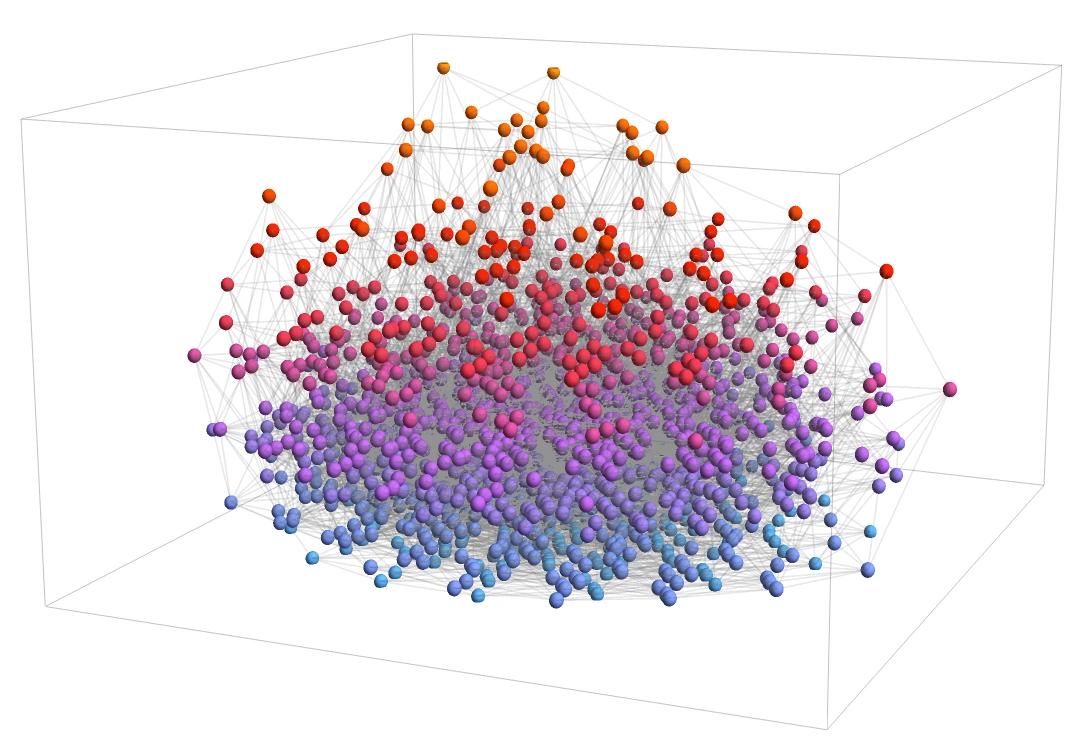
Adaptive evolution should trace a path that never goes downhill:

[Image unavailable: the source image is missing.]

Along this path, derivative-like plots reveal the local terrain at each point and show which available upward direction was actually chosen:

[Image unavailable: the source image is missing.]

The underlying rule space is discrete and high-dimensional; in the case discussed here its dimension is 15. Producing an intelligible three-dimensional picture is challenging. Ideally, rules separated by one mutation would be shown at a fixed elementary distance in two dimensions. That cannot generally be achieved exactly, but a suitable layout of the underlying mutation graph can approximate it.

Given such a layout, we could interpolate between discrete points to form a landscape surface. It is unclear how much meaning to attach to this, but it may appeal to our spatial intuition:

[Image unavailable: the source image is missing.]

Applying machine learning and dimensionality reduction to rule vectors—lists of outcomes not eliminated in the adaptive process—might do slightly better:

[Image unavailable: the source image is missing.]

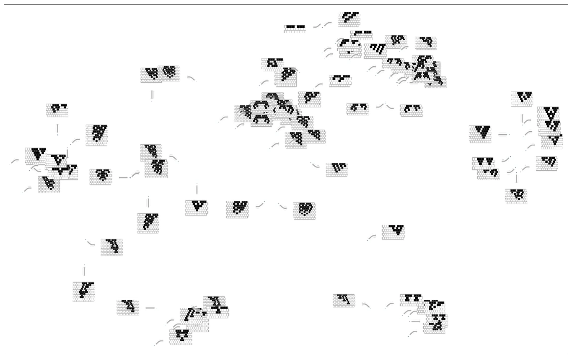
With this dimensional reduction, rule behaviors are distributed as follows:

For comparison, here is a feature-space distribution based on the visual features of the patterns:

[Image unavailable: the source image is missing.]

The whole space: exhaustive search versus adaptive evolution

Adaptive evolution starts with a rule, perhaps the null rule, and tries random mutations to reach rules of progressively greater fitness. What if we exhaustively searched the entire space of possible rules instead? Although rule counts quickly become unmanageable, some cases can be explored:

For symmetric $k=2,r=2$ rules, there are 524,288 possibilities, of which 77,624 generate finite-lifetime patterns. Only 77 distinct phenotypic patterns occur, with differing lifetimes and multiplicities. At least here, multiplicity always corresponds to unused bits in a rule:

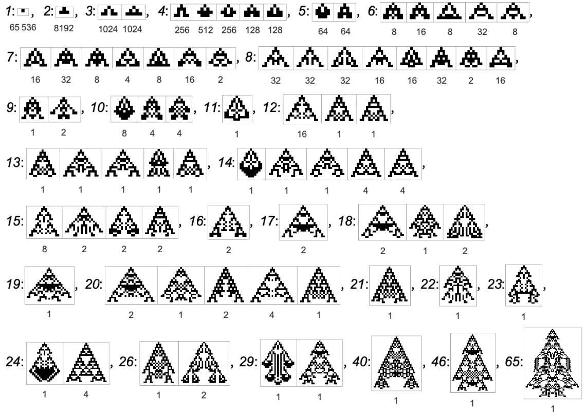
How does this compare with the adaptive multiway graph? The results are almost identical, but exhaustive search adds two cases:

[Image unavailable: the source image is missing.]

They are generated by rules of the following form; gray entries are irrelevant:

[Image unavailable: the source image is missing.]

Why do these rules not appear in adaptive evolution? There is no chain of point mutations from the null rule that reaches them without passing through a rule evolution would reject. A graph containing every acceptable rule has a separate component with its own root, containing rules inaccessible from the null rule:

[Image unavailable: the source image is missing.]

The lifetime distribution across all symmetric $k=2,r=2$ rules is:

[Image unavailable: the source image is missing.]

The maximum shown is 65. The overall distribution is approximately a power law with exponent −3:

[Image unavailable: the source image is missing.]

Not every rule uses every bit, or outcome, when generating its phenotype. Longer-lived patterns, however, generally use more bits:

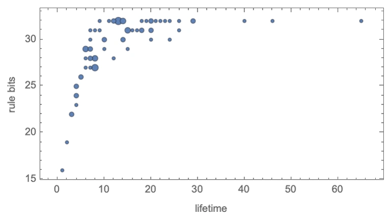
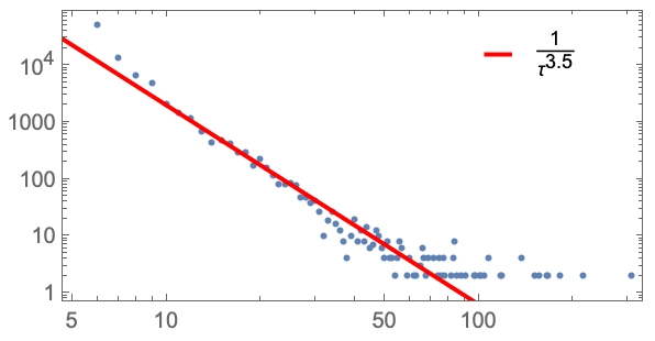
This relationship is also roughly power-law-like, with exponent approximately −3.5:

Here are the 100 longest-lived patterns actually generated. For each asymmetric case, rules also exist that produce its left–right reflection:

[Figure missing in the source note.]

Different rules use fundamentally different ideas to produce these patterns. Some, such as a rule with lifetime 151, seem constructed specifically for their long lifetime. Others, such as one with lifetime 308, appear more accidental: seemingly random behavior simply happens to die out after a certain number of steps.

Because these rules were found exhaustively, we know they are the only ones with such long lifetimes, at least for $k=2,r=2$. To survive more than 100 steps, for example, the complex structures we see are in some sense necessary. When adaptive evolution produces a lifetime beyond 100 steps, the complexity is not the consequence of complicated choices in evolutionary history. There is no alternative but to use a complex pattern. The observed complexity reflects computational necessity rather than historical contingency.

Some behaviors are possible and others are not, as we will discuss in more detail below. A rule can have lifetime 308, for example, while none has lifetime 300. A more complicated initial condition or rule family might make such a lifetime possible.

As in the symmetric case, almost all long lifetimes require every available rule bit:

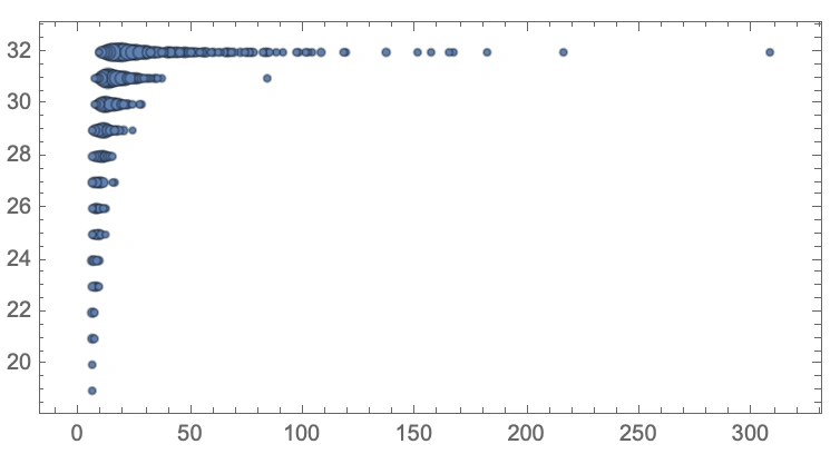
There is, naturally, an exception: a pair of rules with lifetime 84, for which the outcome of case does not matter:

Can these long-lived rules be reached from the null rule by adaptive point mutations? Rather than construct the full forward multiway graph for general $k=2,r=2$ rules, we can build a reverse graph. Starting from a given rule, make all point mutations that lead to progressively shorter lifetimes:

[Image unavailable: the source image is missing.]

At least in this case, the process never reaches the null rule. The furthest it gets is to lifetime-two rules. Among those, the nearest to the null rule are:

[Image unavailable: the source image is missing.]

Yet none of the 26 one-bit rules retained in our adaptive process can reach these two-bit rules by a single point mutation. This is not peculiar to one long-lived rule; it is a general feature of these $k=2$ rules. Building the forward graph from the null rule reaches only rules of lifetime one.

Ultimately, this is a special property of two-color rules and of starting from the lifetime-one null rule. Nevertheless, it shows that large regions of rule space can be inaccessible to adaptive evolution through single-point mutations.

What about symmetric $k=2,r=2$ rules? Preserving symmetry requires mutations that sometimes change two bits rather than one. Apart from the special cases noted above, the reverse multiway system then always reaches the null rule:

[Image unavailable: the source image is missing.]

Another striking feature appears: a single two-bit mutation can take a rule directly from lifetime one to lifetime 65:

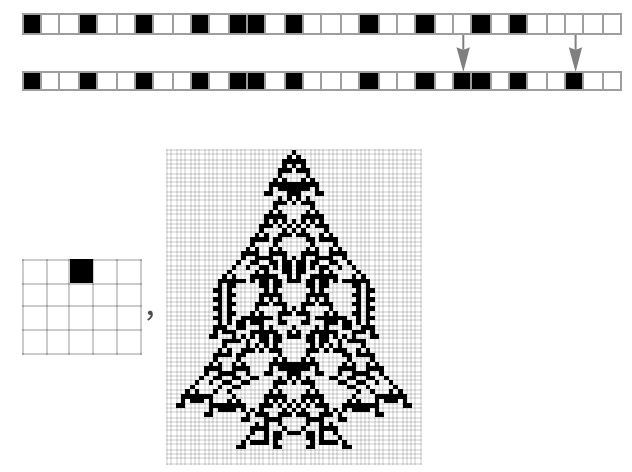
We did not see this in the earlier graph because we applied transitive reduction. Without that reduction, substantial lifetime jumps appear, as illustrated by the distribution of lifetimes before and after a point mutation:

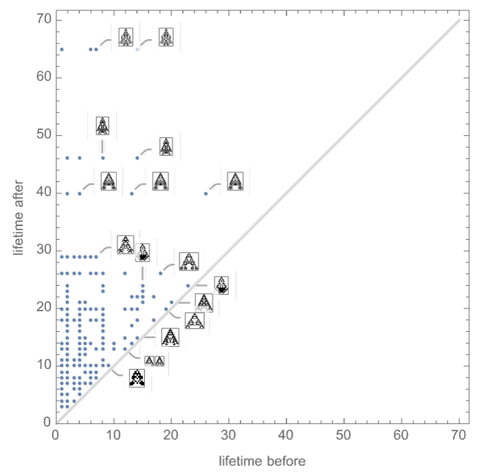
The earlier transitively reduced graph concealed these jumps. Looking at the unreduced distribution makes their size visible:

[Image unavailable: the source image is missing.]

This distribution is again roughly a power law with exponent −3.5:

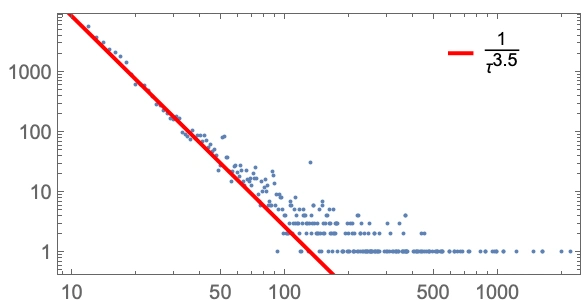
The largest lifetime now found is not merely 308, but 2,194:

[Figure missing in the source note.]

Again we see several distinct ideas at work, together with interesting cases of convergence. Rules with lifetimes 989 and 990, and likewise 1,068 and 1,069, generate effectively the same pattern after a color exchange and an extra initial step.

For general $k=3,r=1$ rules, the space is too large for an easy exhaustive search. Targeted random sampling nevertheless finds many long-lived examples:

[Figure missing in the source note.]

The tail of very long lifetimes extends further:

[Figure missing in the source note.]

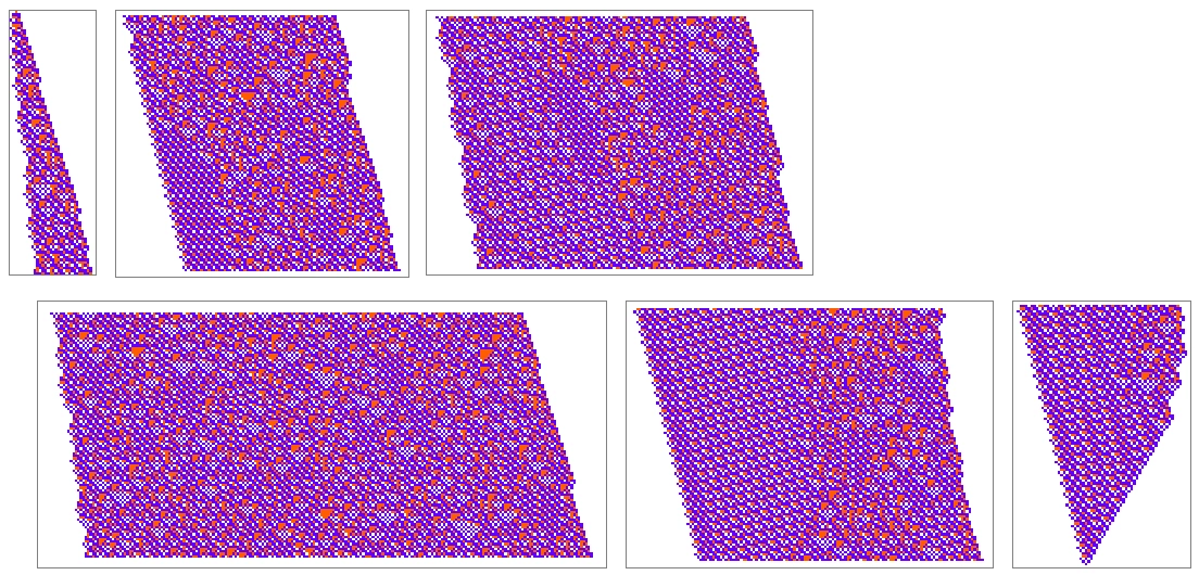
To see the behavior of a rule with lifetime 10,863 more clearly, we can display it in segments and adjust colors for contrast.

Sampling 100 steps every 2,000 steps, together with the final step, reveals alternating complex periodic and apparently random behavior. None of it gives an obvious clue to the remarkable fact that the entire pattern disappears after 10,863 steps:

The issue of undecidability

We have evaluated cellular-automaton fitness by the lifetime of the generated pattern, always assigning zero fitness to patterns that never terminate.

But how do we determine whether a pattern will terminate? The previous section included patterns that lived a very long time before disappearing.

Here are the first 100 steps of patterns generated by some symmetric $k=3,r=1$ rules:

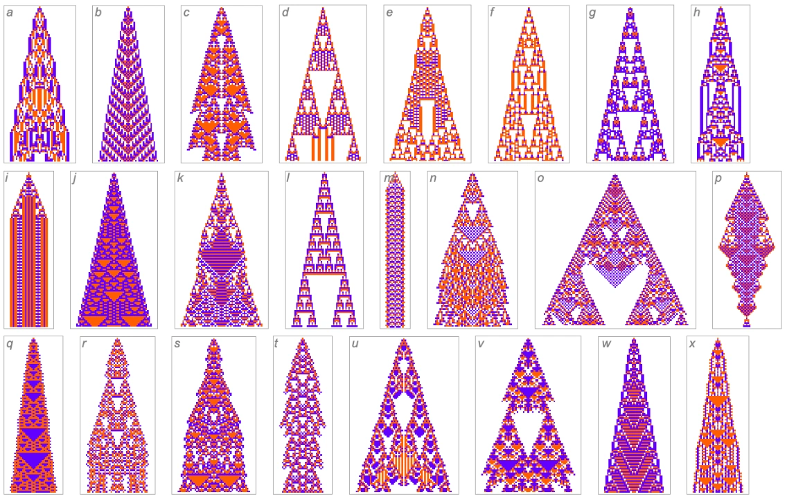
What will happen? We know only that their lifetimes are at least 100 steps. To infer more, we need additional information. A periodic pattern, or an obvious repeating structure, may reveal that it will never terminate. In other cases, there is no obvious way to predict what comes next.

Explicitly running the rules for another 100 steps reveals more:

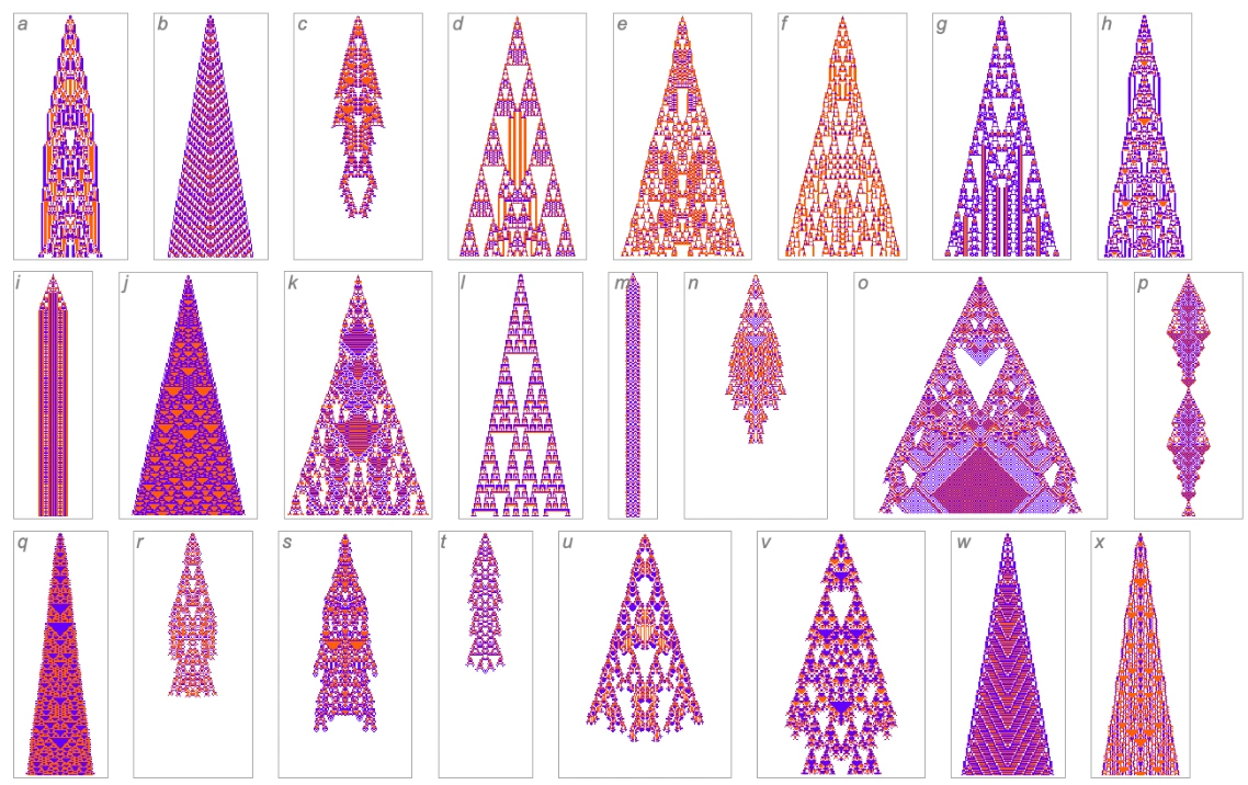
At 500 steps there are surprises. Rule (a) becomes periodic after 388 steps; rules (o) and (v) terminate after 265 and 377 steps:

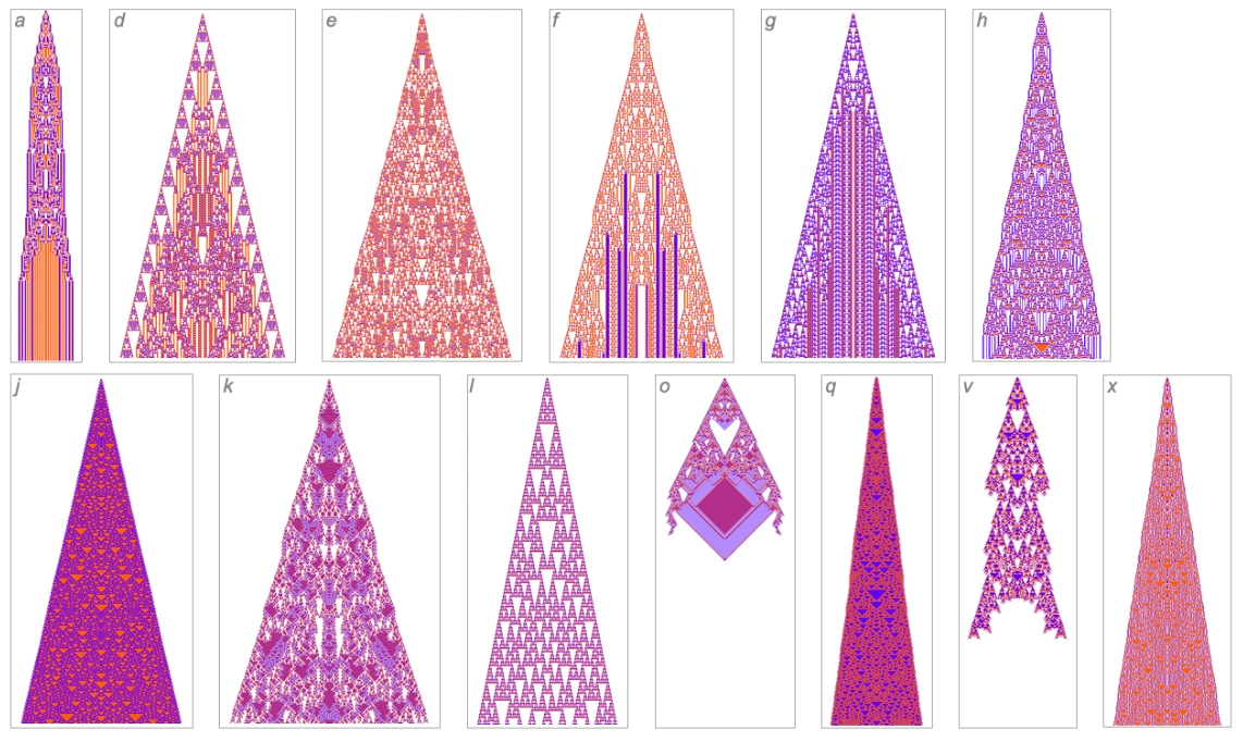
Can we systematically determine what will ultimately happen to all remaining rules? In general, no. This must be regarded as an undecidable problem, not solvable in every case by finite computation.

Because the rules are relatively simple, we might expect sophisticated mathematics and computation to outpace them and determine their outcomes with less work than explicitly following every step.

The Principle of Computational Equivalence, however, says that whenever behavior is not obviously simple, its computational sophistication will be equivalent to that of other systems, including whatever method we might use to predict it. The result is computational irreducibility: in many systems, presumably including most of these automata, there is no more efficient way to find the outcome than to trace the steps. Knowing what happens ultimately, after arbitrarily many steps, can therefore demand unbounded computational effort. No finite computation provides a general decision procedure.

In practice, we may inspect a family’s lifetime distribution and become fairly confident that no greater finite lifetime occurs. For the $k=3,r=1$ rules of the previous section, a few thousand steps might have seemed close to the limit—until the 10,863-step example appeared.

Suppose a rule has run for 10,000 steps without disappearing. How can we establish that it never will? We need a proof. That is easy if the pattern becomes exactly periodic. Usually computational irreducibility prevents such a shortcut, but special cases may permit one. These correspond to pockets of computational reducibility, where we find a compressed account of the behavior.

Some patterns are not strictly periodic as a whole, yet eventually exhibit essentially repeating behavior. This example has period 480:

[Image unavailable: the source image is missing.]

Other patterns are nested and never periodic, but simple enough to predict:

[Image unavailable: the source image is missing.]

Surprises remain. This one eventually settles into period six, but only after 7,129 steps:

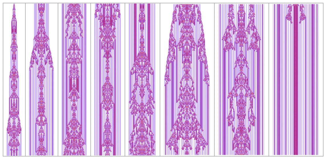
For adaptive evolution, this means we may mistake a very long finite lifetime for an infinite one. In biological terms, a genome might appear to produce unlimited, tumor-like growth, although the growth would eventually stop unexpectedly.

Computation-theoretic perspectives and busy beavers

The question of whether a cellular-automaton pattern dies out directly parallels the Turing-machine halting problem, termination in term rewriting, Post tag systems, and related questions. Searching for automata with the longest-lived patterns is a cellular-automaton analogue of the busy-beaver problem for Turing machines.

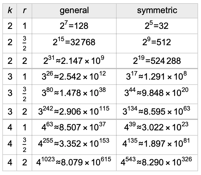
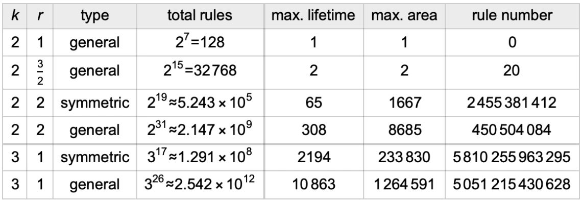
Here is a summary of the results found so far, all for single-cell initial conditions:

The profiles of the patterns—their widths in nonzero cells—are:

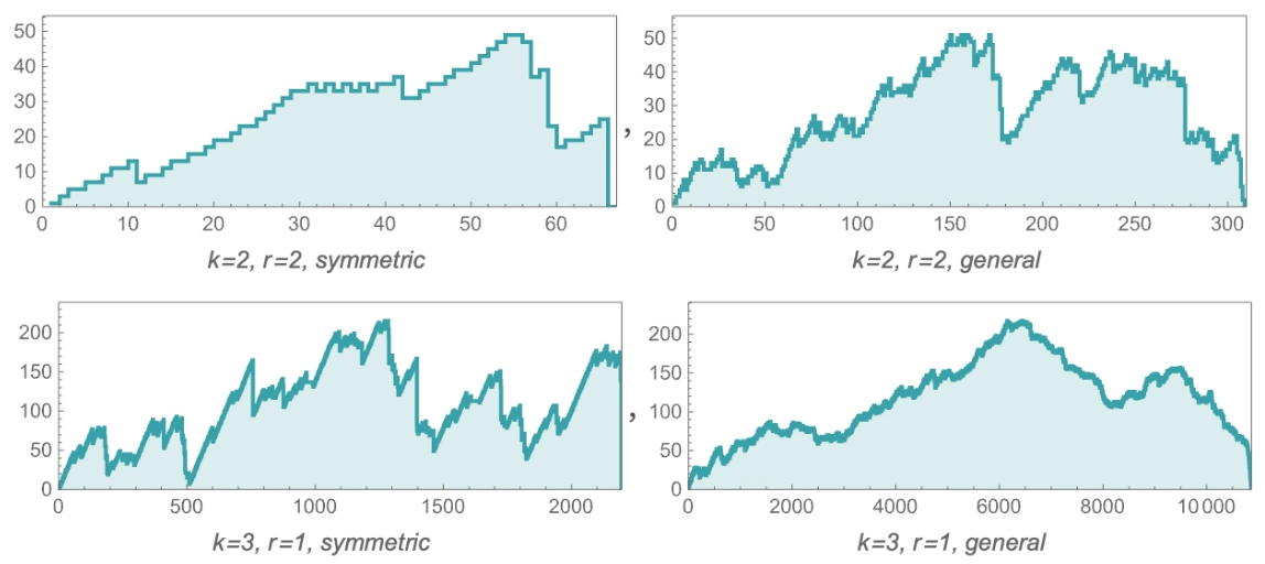
Integrating these curves gives the areas in the table.

As described above, we can be certain only of lower bounds on the true maximum lifetimes, although for all but the last few entries it seems very likely that the maxima have been found.

It is sobering to compare known busy-beaver lifetimes for Turing machines. Here $s$ denotes the number of states; machines start on a blank tape and halt when they reach a specified halting state:

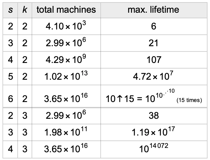
Very small Turing machines may have moderate lifetimes. Slightly larger ones can have vastly greater lifetimes. The undecidability of the halting problem implies that the maximum lifetime eventually grows faster than any computable function of machine size—any function a Turing machine can compute in finite time, or whose values can be established by finite proofs within a finite axiomatic framework.

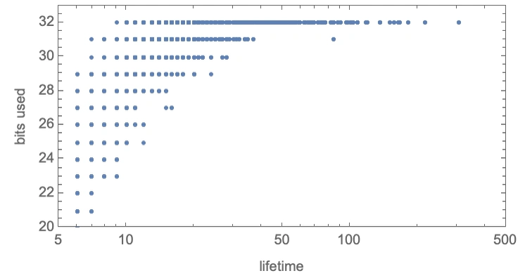
Maximum lifetime thus grows with rule size, whether for Turing machines or cellular automata. What defines that size? Presumably it is approximately the number of independent bits needed to specify a rule—an approximate measure of information content—or the base-two logarithm of the number of rules in its family.

We might initially think all $2^{32}$ rules with $k=2,r=2$ require 32 bits each. As noted above, however, some bits can be irrelevant to the pattern generated. The more bits matter, and thus need specifying, the longer the lifetimes that can be achieved:

So far, we have considered single-cell initial conditions. More complicated initial conditions add information to the system and can increase its maximum lifetime. For example, here are lifetimes available to $k=2,r=\frac{3}{2}$ rules across a range of possible initial conditions:

[Image unavailable: the source image is missing.]

Probabilistic approximations?

Cellular automata are deterministic: a rule and an initial condition completely determine every aspect of their behavior. Could some probabilistic model approximate that behavior? Or could such a model at least describe aggregate properties across many rules?

One clue may lie in the power-law distributions of lifetime frequencies found above. Can a probabilistic model account for those distributions, perhaps even their exponents?

We could approximate an automaton by a probabilistic process in which a cell becomes black with probability $p$ if it or either neighbor was black on the previous step. Here are examples of this directed-percolation setup:

Behavior varies greatly with $p$. For small values everything disappears; for larger ones the pattern fills space:

Starting from a random initial condition, the eventual density shows a clear phase transition near $p=0.54$:

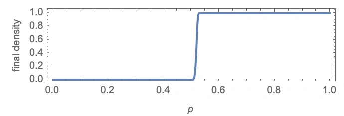
Starting instead from a single black cell gives a slightly different transition:

[Image unavailable: the source image is missing.]

We can plot the probabilities of different survival times or lifetimes:

[Image unavailable: the source image is missing.]

Near the transition, the lifetime distribution is roughly the power law $\tau^{-1}$, which also happens to be the mean-field-theory estimate.

How does this relate to cellular automata? For a $k=2$ rule, suppose cell colors can be approximated as random. The generated pattern might resemble this probabilistic model, with $p$ related to the fraction of rule cases that output black.

Plotting $k=2,r=2$ lifetimes against these fractions, we find that the longest lifetimes occur near one-half black outputs. Note, however, that the binomial distribution also places the greatest number of rules there:

[Image unavailable: the source image is missing.]

Rather than describe the detailed evolution, we might approximate the boundaries of finite-lifetime patterns—say, symmetric ones—as random walks. Their collision marks the pattern’s disappearance:

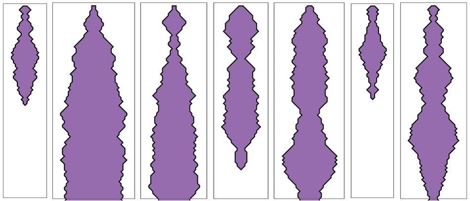
Standard random-walk theory gives a large-$\tau$ lifetime probability proportional to $\tau^{-3/2}$. That is a power law, but not the one observed for the cellular-automaton lifetimes.

Other adaptive-evolution strategies

So far we have always accepted outcomes of equal or greater fitness. What if a more impatient procedure demanded a strict increase at every step?

For $k=2$, it cannot escape the null rule at all, at least from the starting condition considered: every pattern reachable in one mutation still has lifetime one. For $k=3$, one improving mutation is possible, but no more, as this multiway graph shows:

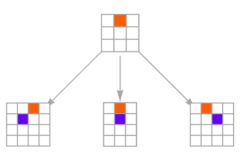
That assumes improvement must occur in a single mutation. Allowing two mutations at once enables progress. Here is the graph for symmetric $k=2,r=2$ rules:

[Image unavailable: the source image is missing.]

It does not reach as many phenotypes as single mutations with neutral moves, but reaches the accessible ones faster, without wandering back and forth through neutral space.

Allowing up to three mutations extends the reach:

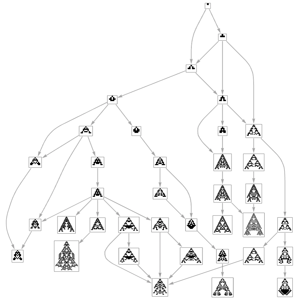
This seems a reasonably representative sample, despite reaching only 37 rules rather than the 77,624 accessible under the standard neutral-move procedure, many of which share phenotypes.

For symmetric $k=3,r=1$ rules, single mutations allow two steps:

[Image unavailable: the source image is missing.]

Allowing up to two mutations goes farther. Without having to handle neutral moves, we can explicitly construct at least the first few stages of the graph:

These two-mutation moves thus make more of the initial multiway structure directly accessible:

The histories just shown can be generated by trying possibilities at random and choosing the first that improves fitness. Another strategy is local exhaustive search: examine every possible mutation at each step and choose the greatest fitness increase. In smaller rule spaces, several choices often have equal fitness, so we can choose randomly among them:

[Image unavailable: the source image is missing.]

One might expect this to optimize evolution. Its systematic nature, however, can leave it stuck, repeatedly trying the same thing even when that fails.

An almost opposite strategy loosens selection, allowing paths that temporarily reduce fitness—for example, lowering lifetime by one step:

We are allowing less-than-maximally-fit individuals to survive. The corresponding multiway graph includes backtracking to lower fitness:

[Image unavailable: the source image is missing.]

Although details differ, allowing this backtracking does not appear to have a dramatic overall effect. The basic phenomena seem robust enough that many details of the adaptive procedure do not ultimately matter.

An aside: sexual reproduction

So far, mutations have operated on one rule at a time. Many organisms also use sexual reproduction, combining a pair of rules—or genomes—to make a new one. As a simple model of genomic crossover, join the beginning of one rule to the end of another:

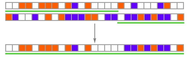
Usually there are many ways to combine a pair. In a direct analogy with our Physics Project, a recombination can be represented as an event that consumes two rules and produces a new one:

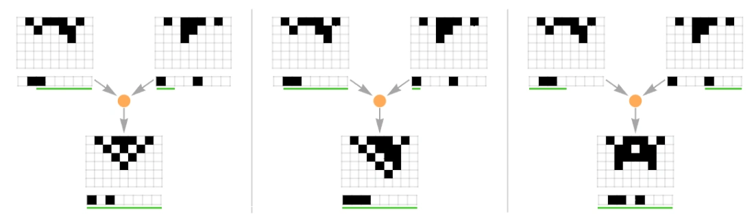
The counterpart of the multiway graph of all possible adaptive histories is now what we call a token-event graph in the Physics Project:

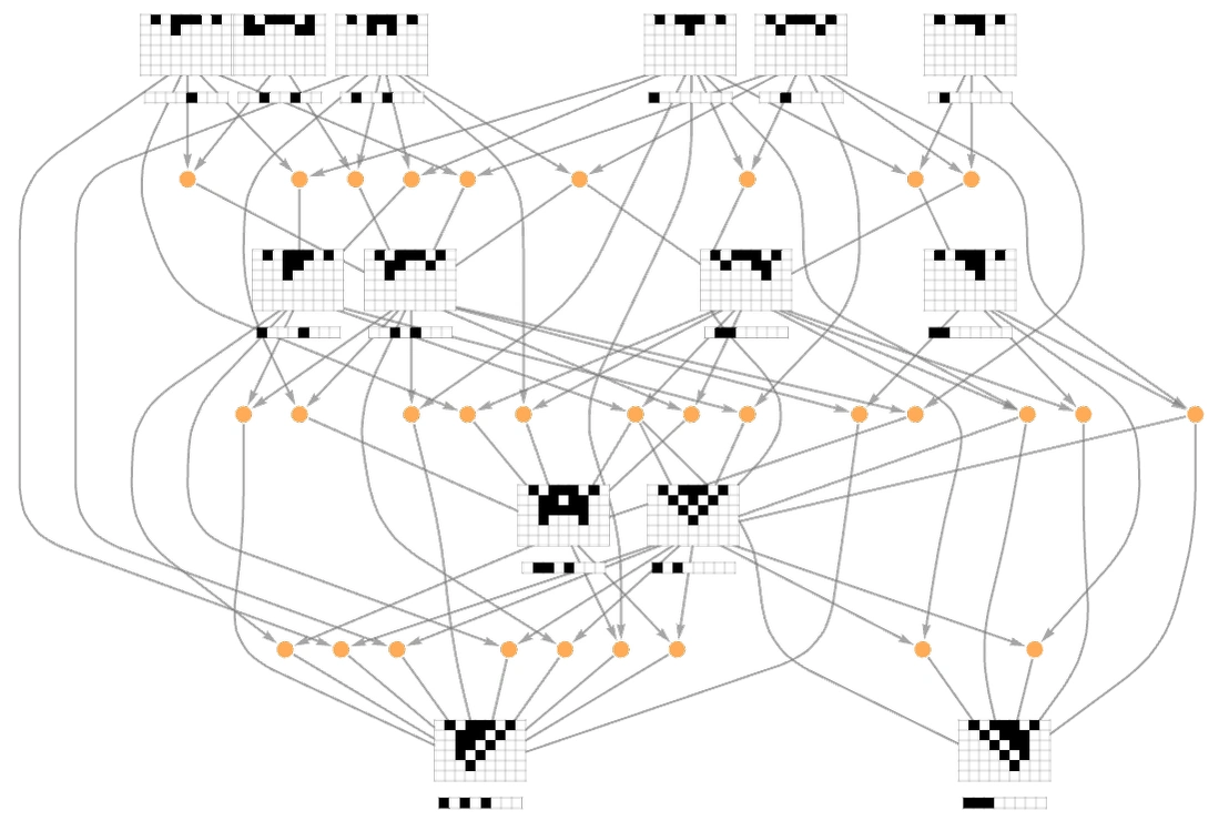
With mutations alone, we could start from one rule and modify it step by step. Now we need a population of rules, repeatedly combining pairs to produce new ones. Possible pairings can be represented as:

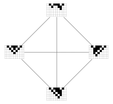
There are many modeling choices. In this particular version, choose $n$ possible pairings from the $n(n-1)/2$ available:

[Image unavailable: the source image is missing.]

For each selected pair, try crossover and retain offspring not rejected for lower fitness. Here, offspring are represented by lines joining their parents:

[Image unavailable: the source image is missing.]

Finally, to maintain the gene pool, randomly carry some parents into the next generation so the population again contains $n$ rules. Despite our attempt at minimalism, this becomes rather messy—apparently unavoidably so, and, as discussed below, a recurring difficulty in evolutionary-computation research.

Apply this to $k=3,r=1$ rules, choosing four random rules as the initial population. Two happen to generate the same pattern:

[Image unavailable: the source image is missing.]

Across successive steps, different pairs are selected:

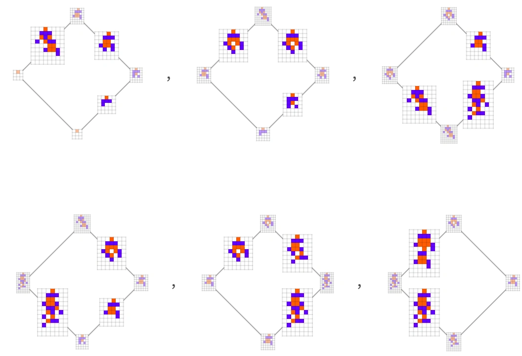
Here are the distinct phenotypic patterns that arise. Several copies of a phenotype can occur, while their underlying genotypic rules remain different:

[Image unavailable: the source image is missing.]

A summary plots the successive fitness values, with point size indicating how many times a fitness occurs:

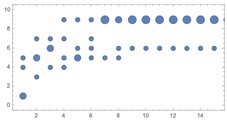
Here a steady state appears after nine steps. Larger populations generally continue evolving longer. Two examples with population ten show all patterns obtained:

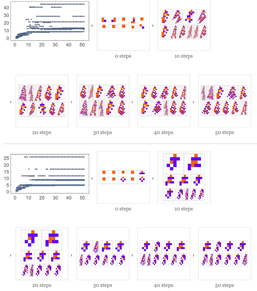
Keeping only each case’s longest-lived rule found so far gives:

[Image unavailable: the source image is missing.]

The results do not look clearly different from mutation-only evolution, despite the more elaborate population-based model. One obvious distinction is that entire rule populations can cycle. Under pure mutation, cycles occur only among fitness-neutral rules.

Here are further examples from populations of 25 after 500 steps:

[Image unavailable: the source image is missing.]

And with population 50:

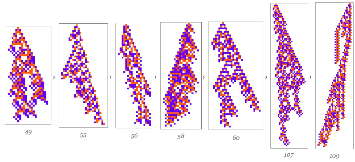
Even here, no major difference from mutation-only results is apparent. Sexual reproduction and crossover introduce details, but to understand the broad character of adaptive evolution, considering mutation alone seems sufficient.

An even more minimal model

Cellular-automaton evolution is already a dramatic simplification of real biology. To understand the essential phenomena, however, we can simplify further. Instead of computational rules and their behavior, consider vertices on a mutation graph, each assigned a fitness.

For example, assign a random fitness to every point on a two-dimensional grid:

[Image unavailable: the source image is missing.]

Starting at a minimum-fitness point, follow the same adaptive procedure: move at each step to a neighboring point with equal or greater fitness:

[Image unavailable: the source image is missing.]

Usually we get stuck before going far, although with the uniform fitness distribution used here, the final value is generally relatively high.

A multiway graph summarizes possible paths:

[Image unavailable: the source image is missing.]

In cellular-automaton rule space—and more broadly in biology—neighbors do not have independent random fitnesses. A definite computation determines fitness. As a simple approximation, let fitness be a particular function of graph coordinates. If it forms a smooth hill, adaptive evolution climbs it:

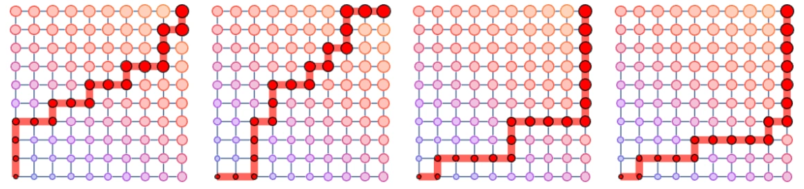
Once the function has systematic undulations, however, the process strongly tends to get stuck quickly:

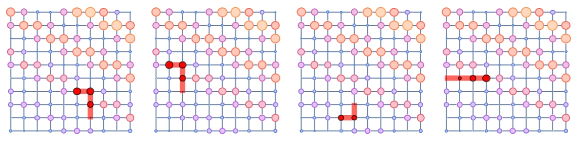
An unexpectedly high-fitness point is usually not found, and is certainly unreachable if surrounded by a moat of lower fitness:

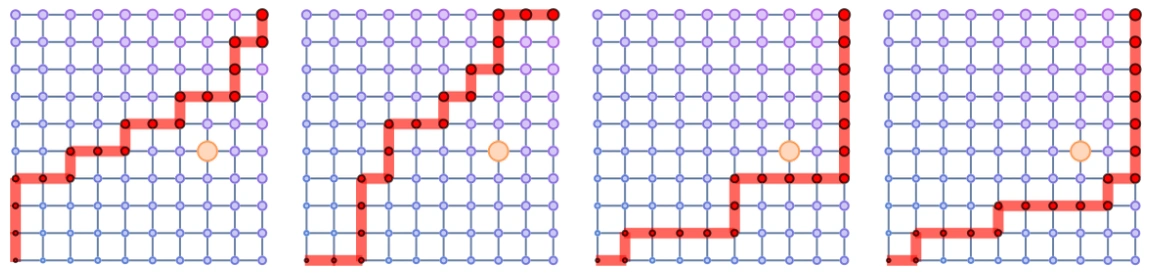
Increasing the mutation space’s dimension makes it easier to find an improving path:

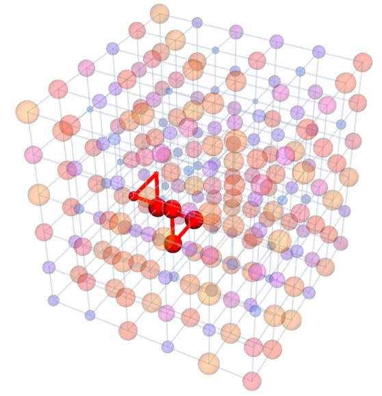
Boolean hypercubes of increasing dimension illustrate this:

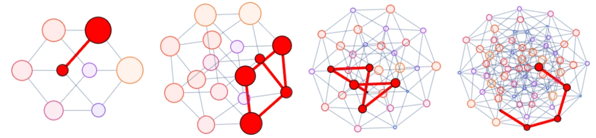
The key is that the neighborhood accessible by mutation contains a sufficiently random collection of fitnesses, making an upward direction likely. Usually that alone is insufficient. The landscape must also have enough regularity to navigate systematically toward a maximum, rather than leaving that maximum as an isolated surprise.

What can adaptive evolution achieve?

Adaptive evolution can be surprisingly successful at discovering automata with long but finite lifetimes. What about other characteristics? What can it ultimately do, and what can it not do?

Suppose we seek patterns that die after an exact number of steps rather than simply live as long as possible. Any finite rule family—such as fixed $k$ and $r$—has only finitely many attainable lifetimes. For symmetric $k=2,r=2$ rules, they are:

For symmetric $k=3,r=1$ rules, every lifetime up to 100 is possible in principle. How well does adaptive evolution find them? Keep point mutations, but accept them when they bring the lifetime closer in absolute difference to a specified target. Crucially, as before, neutral mutations that leave the fitness unchanged are also accepted.

Here are attempts to evolve $k=3,r=1$ rules with lifetime exactly 50:

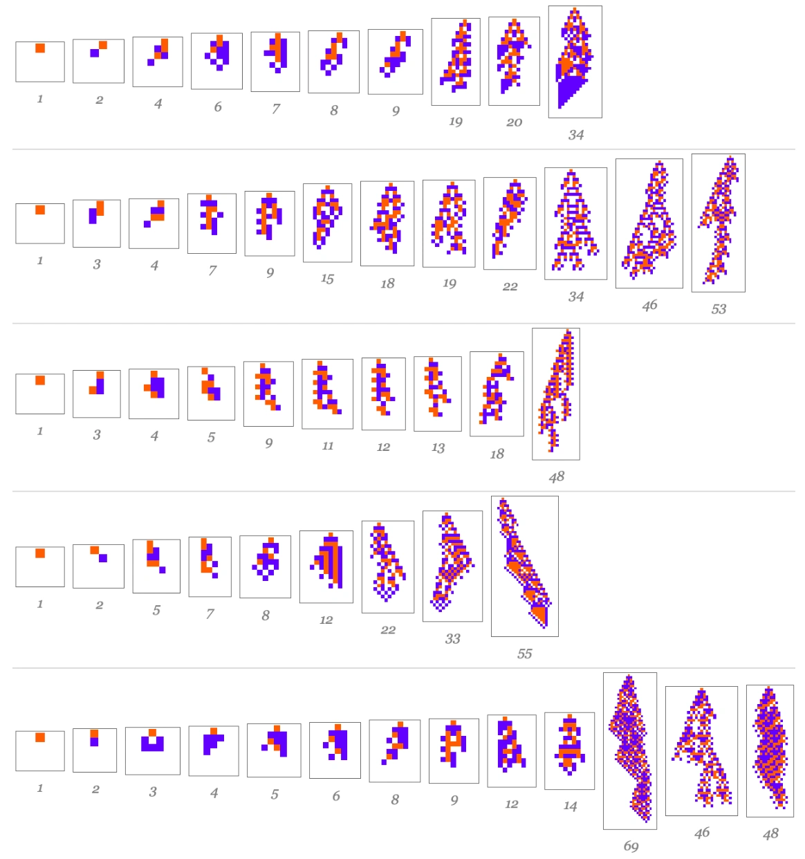
They approach the target, sometimes overshooting it, but these examples never hit it exactly. Across 100 random mutation sequences, the attained lifetimes are:

[Image unavailable: the source image is missing.]

Most settle near 50 rather than at it. This is not because the rule family cannot produce lifetime 50. Exhaustive search finds many such rules, even symmetric ones:

[Image unavailable: the source image is missing.]

The adaptive process usually gets stuck before reaching them. The rule space generally has enough room to maneuver toward longer lifetimes, but not enough to reliably reach this exact target.

What about $k=4,r=1$? The space now contains roughly $10^{38}$ rather than $10^{12}$ rules. Lifetime 50 becomes a fairly common adaptive outcome:

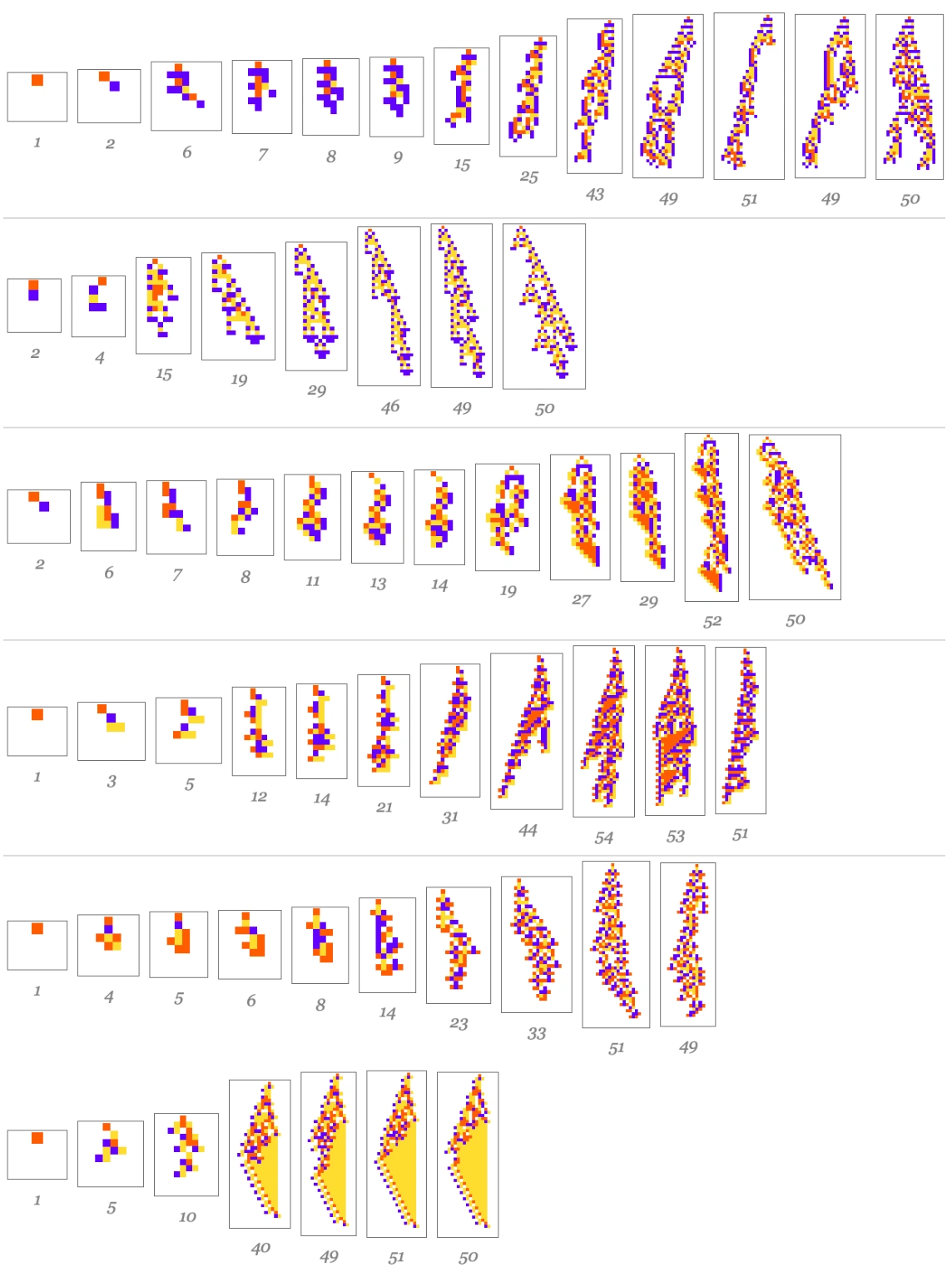
It may take time, but most cases now reach exactly 50:

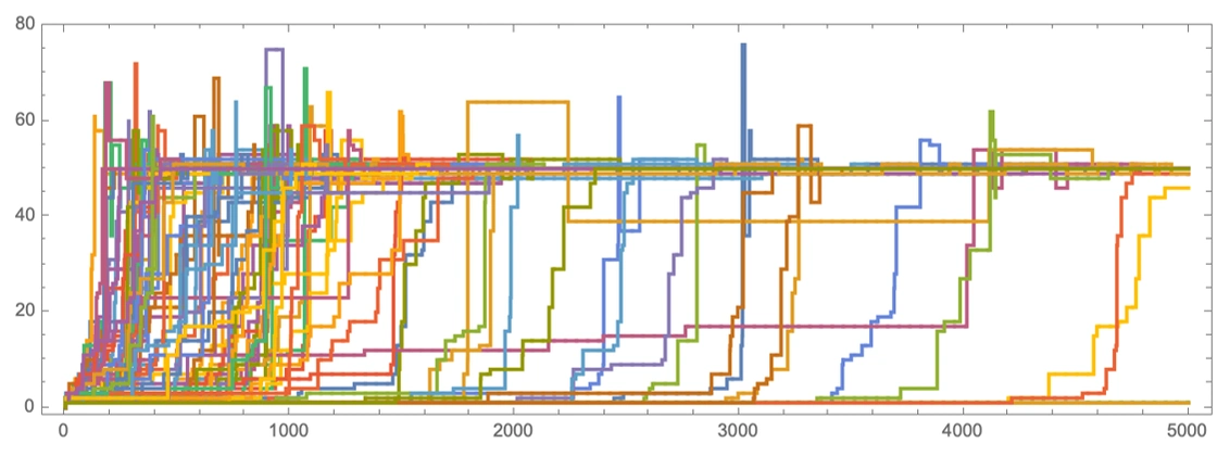
What about other targets? Even symmetric $k=3,r=1$ rules can attain many different lifetimes:

[Image unavailable: the source image is missing.]

The first missing values are 129, 132, 139, and so on. Many multiples of 50 are possible:

[Image unavailable: the source image is missing.]

Yet finding a particular target becomes harder. Increasing rule-space size seems consistently helpful. For $k=4,r=1$ and target lifetime 100, the achieved distribution is:

[Image unavailable: the source image is missing.]

Distributions generally broaden as target lifetimes increase:

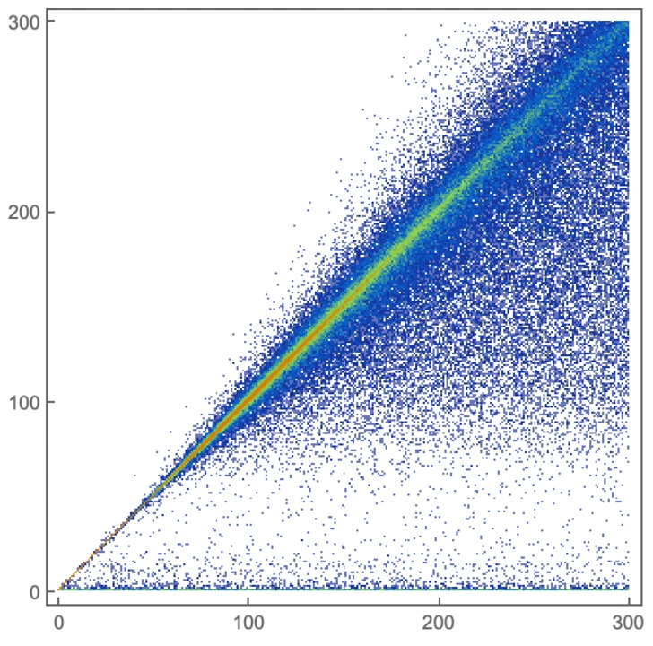
Longer lifetimes in spaces such as $k=4,r=1$ occur with approximately power-law frequencies. Regions achieving a given lifetime therefore become progressively smaller, and evolution is increasingly likely to get stuck before reaching them.

What about morphological objectives? Consider maximizing the width of finite-lifetime patterns. Reject mutations that reduce width, defined as the maximum horizontal extent. Again, evolution discovers varied mechanisms to increase it. Here patterns are labeled by height, or lifetime, and width:

[Figure missing in the source note.]

Structural constraints apply. Width cannot be too large relative to height, because overly broad patterns tend to grow forever.

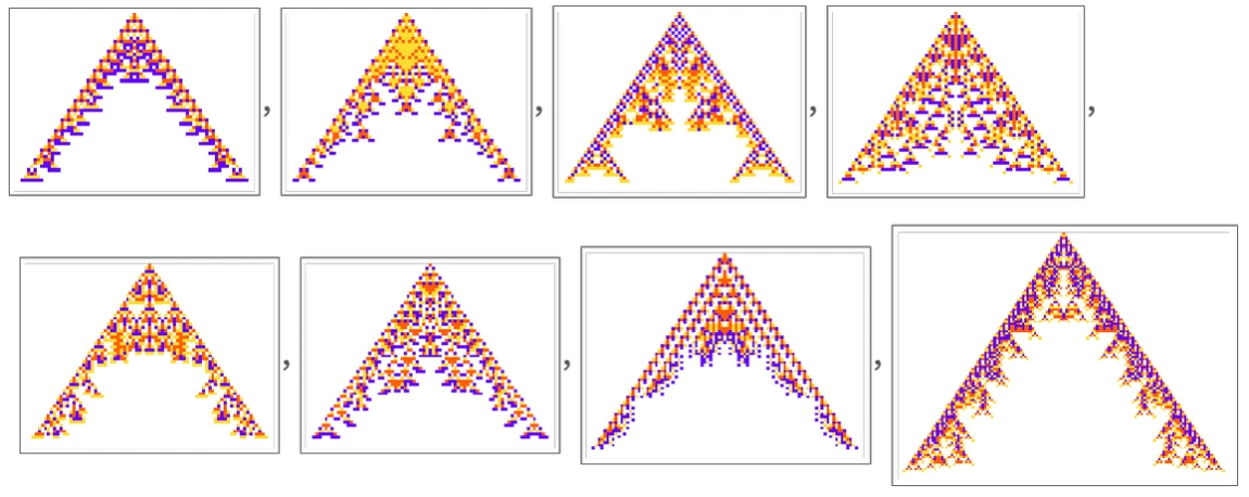
What if we maximize the width-to-height aspect ratio itself? In most earlier examples, evolution invented many mechanisms for the objective. Here it repeatedly uses the same idea, presumably because the rule family’s overall structure leaves effectively only one way to achieve it:

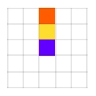
Demand an aspect ratio as close to three as possible, and the solution is usually correct but obvious:

Sometimes another solution appears, often unexpectedly intricate:

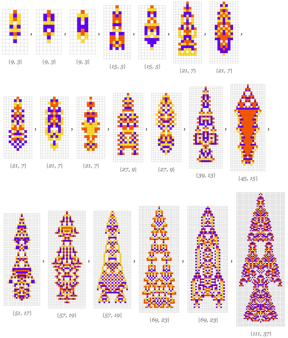
For an aspect ratio near $\pi\approx3.14$, even symmetric $k=4,r=1$ rules do fairly well:

[Image unavailable: the source image is missing.]

We can also target properties inside a pattern—for example, maximize the length of a constant-color run of nonwhite cells in its center column. Adaptive evolution again finds rules with large values, such as these random examples:

[Image unavailable: the source image is missing.]

We could ask for exact run lengths or the presence or number of particular subpatterns. Eventually, as with very long lifetime targets, the desired outcomes become too sparse for adaptation to find them in a given rule space, even though exhaustive search can still identify examples.

Which goals or fitness functions are well handled by evolution operating on raw material such as cellular-automaton rule space? This is important, and its counterpart is fundamental in machine learning. We do not yet have adequate tools to answer. It resembles asking which functions different methods or basis functions can approximate, and how well, but is more complicated. An answer would tell us much about adaptive evolution’s reach, with consequences for both biology and machine learning.

What this means for biology

How can organisms exist as they do, solving so many challenges with seemingly sophisticated and ingenious solutions? Did natural selection do everything, or is something else involved? If selection did it, how?

From traditional engineering’s perspective, biology is often surprisingly complex and clever, perhaps beyond what we could create ourselves. Is natural selection its entire secret? Engineering also involves selection-like processes: different designs are tried and only some retained. A key distinction, though, is that traditional engineers usually try to foresee a design’s consequences.

Biology is different. Genomic mutations occur randomly, without foreknowledge of their effects. Still, one might assume that selection would guide the result toward something resembling traditional engineering.

A crucial intuition is missing: how do randomly chosen programs behave? Based on experience constructing programs for specific purposes, we might expect simple random programs never to do anything especially interesting or complicated.

My discoveries in the early 1980s showed that expectation to be wrong. In the computational universe of possible programs, very simple ones can generate enormous complexity. Mutations acting on genomes will therefore inevitably sample programs exhibiting highly complex behavior. Such complexity might initially seem possible only through careful design, and rare even then. Surprisingly, the computational universe makes complexity relatively easy to obtain.

How does complexity relate to a successful organism? To thrive in a particular environment, an organism needs a genome that solves the necessary problems. Natural selection enters here, but its effectiveness is far from obvious.

There are two questions: does a program, or genome, exist that solves the required problem? And can a path of adaptive evolution find it while passing only through intermediates fit enough to survive? Both questions are closely linked to the same fundamental computational properties responsible for widespread complexity.

Within a framework such as cellular automata or the basic architecture of life, do rules exist that achieve a particular computational objective? The Principle of Computational Equivalence suggests that the answer is usually yes. Almost any underlying hardware can support software—rules—achieving almost any physically possible goal, such as developing an organism that survives in a given environment. How do we find those rules?

Exhaustive search is possible in principle, but exponentially difficult and practically hopeless beyond toy examples. What about adaptive evolution? That is the central question. What we have seen is that simple mutation and selection—the mechanism of natural selection—often provide a surprisingly substantial shortcut.

Why? Evolution seeks a path through rule space to the desired destination, yet does so one step at a time. It tries random mutations, accepts one that does not decrease fitness, and continues. It is not initially evident that this should work. All directions could eventually reduce fitness, trapping the process.

Our simple-model experiments suggest that this usually does not happen. Two things seem important. Rule space is high-dimensional, leaving many directions in which to advance. But dimensionality is not enough: directions might be correlated, so that blocking one would inevitably block all others.

Why does that not happen? Computational irreducibility appears to be the reason. Traditional intuition from mathematical science suggests that knowing a system’s underlying rules allows immediate prediction of its behavior. My explorations in the 1980s and 1990s instead suggested that, throughout the computational universe, the only systematic way to determine most systems’ behavior is to run their rules step by step and perform the corresponding computational work.

Observing behavior does not therefore allow us simply to decode it and see its simple origins. Unless we perform as much computation as the system itself, we encounter its behavior as effectively random. This appears fundamental to phenomena such as the second law of thermodynamics, and I suspect it is also central to the effectiveness of adaptive evolution, particularly in biology.

Computational irreducibility supplies an effective randomness in the fitnesses around every point in rule space. In a space with many dimensions, a successful onward path is then highly likely.

Can evolution find it? We assume mutations are random. With $n$ elements in a rule, a number of mutations proportional to $n$ should locate a successful direction, whereas exhaustive search requires trying roughly $k^n$ rules.

One might imagine a mutation sequence cleverly probing rule-space structure to identify successful directions. But the mapping from genotype to behavior, or phenotype, is generally computationally irreducible. Computationally bounded mutation generation cannot defeat that irreducibility, so it encounters fitness variations as effectively random.

What about the features an organism needs? It seems essential that, in some sense, they are computationally simple. We require it to live long enough, grow tall enough, or satisfy another coarse criterion—not perform some particular computationally irreducible task. Its development and behavior can involve irreducible processes, but selection ultimately depends on a comparatively simple fitness measure. Biological evolution resembles, in the sense of my recent observer theory, a computationally bounded observer examining an irreducible underlying process.

To that observer, simple laws of evolution appear, together with the idea that natural selection can successfully generate a variety of features.

This has implications for where biological complexity comes from. Does selection produce it, perhaps encoding the complexity of a historically contingent mutation sequence? Or does it arise elsewhere?

In this picture, it largely arises elsewhere, reflecting computational irreducibility. The capacity to generate organisms with such varied forms and functions comes from the universal computational character of the underlying architecture, closely tied to irreducibility.

Because selection acts so coarsely, it does not avoid the irreducibility widespread in rule space. Looking deeply into biological systems, we therefore tend to encounter irreducibility and its associated complexity.

We have repeatedly seen evolution solve a problem in a way that looks extraordinarily complicated to us. A simple engineering solution might exist—for example, using highly regular behavior—but that is not what evolution finds. Its solution is often surprising:

[Image unavailable: the source image is missing.]

Adaptive evolution may thus lead to characteristically special regions of rule space, suggesting a characteristic specialness in the structures biological systems produce. A general account of that specialness could offer a framework for a new, broadly formulated theory of biology.

Correspondence with biological phenomena

Our models are extremely simple in their construction. It is somewhat surprising that, without including biophysics or biochemistry, they nevertheless capture features of biological systems and evolution.

Ultimately this reflects biology’s computational character and the universality of computational phenomena. Yet even the patterns produced by cellular automata look strikingly lifelike and organism-like.

Real genomes, even the shortest, are much longer than our small rules. But a genome sequence of length 27, as in a $k=3,r=1$ automaton, already has around 30 trillion possibilities—apparently enough to exhibit many core combinatorial biological phenomena.

Running an automaton rule may seem remote from making organisms through proteins and complex functional and spatial structures. More analogies exist than one might expect. Particular rule cases are generally used only in particular regions of a developing pattern, much as particular genes are activated in different tissues.

With sophisticated computation, geometrical restrictions to one-dimensional arrays of cells also seem less consequential. Many structures still closely resemble those arising as organisms grow.

Self-reproduction is a defining feature of organisms. Without copying there would be no adaptive evolution to discuss. Our models do not derive self-reproduction; they build it in.

Mutation is likewise built in, despite the variants considered. Single point mutations occurring one at a time appear sufficient to capture the essential adaptive phenomena.

We have mainly considered a single lineage, with one rule or genome at each step. We mutate it and implement selection chiefly by retaining rules that produce fitter patterns.

A full population may not be essential, but in our simple setting it is important not to exclude neutral mutations. Repeatedly, a system wanders through a neutral region of rule space before discovering an innovation that raises fitness. This wandering always changes genotype but often changes phenotype only slightly. Long periods of apparent equilibrium, with little phenotypic change, are followed by jumps to new fitness levels and very different phenotypes.

This seems closely aligned with the punctuated equilibrium often reported in the fossil record.

Another central feature of life is the formation of species, phyla, and other groups. Our multiway graphs commonly show an apparent analogue: adaptive paths branch into groups using different computational mechanisms to achieve fitness.

Real biology has many details involving reproductive and spatial isolation. In our models, however, the core cause of branching in the tree of life seems to be the existence of different computational mechanisms in different parts of rule space. Branches can also die out, leaving no subsequent species in the graph.

Examining the patterns generated in different graph regions, one can readily imagine a morphological taxonomy resembling, though not exactly matching, the phylogenetic tree defined by mutations. Morphological convergence occurs often. Small models sometimes even show genomic convergence, which would generally be astronomically rare in real biological systems.

A notable strength of these models is their fairly comprehensive view of whole evolutionary histories. Small rule spaces often reach their highest attainable fitness after relatively few mutations. Yet, as Turing-machine examples suggest, a modest increase in rule size can allow evolution to go vastly farther.

Farther along, more mechanisms are invented. Irreducible computation inevitably brings new and unpredictable phenomena, while new pockets of reducibility also keep appearing. Thus, even after billions of years, trillions of generations, and roughly $10^{40}$ organisms, evolution still has endless room to continue, creating new branches of life with new mechanisms.

One might imagine organisms eventually attaining maximum fitness and stopping. But even our simple lifetime-based model has no ultimate fitness ceiling: for any given lifetime, basic computation theory implies that a program can exist with a longer one. We might say enough is enough—a giraffe’s neck is already long enough. Competition nevertheless keeps things moving: when another lineage reaches the same fitness, the first must advance to avoid falling behind.

Our simple models do not explicitly include interactions among organisms, detailed environments, or countless other influences. Many biological phenomena undoubtedly depend on them. The important point is that many central evolutionary features appear even without them. Biological evolution—and adaptive evolution more generally—seems fundamentally computational, robust across system details.

Our Physics Project has, in recent years, provided strong evidence for computational foundations of physics: its central laws emerge from how observers like us parse the ruliad of all possible computations. We now see remarkable common ground between physics and biology. Both are rooted in computational irreducibility and both sample reducibility. Physics does so because bounded observers need descriptions of the world; biology does so because selection pursues coarse objectives.

Physics encourages the intuition that simple models ultimately exist. Biology often seems almost infinitely complicated, with a new effect at every turn. Perhaps much of the difference is that biological subjects quickly confront irreducibility, whereas physics has found subjects that avoid it. Their shared foundations suggest that biology, too, should possess structures and general laws supporting useful, broad statements. The simple models proposed here may help point toward a new paradigm for fundamentally theoretical biology.

Historical background

This discussion has a long and winding history. Basic ideas of heredity were widely recognized in antiquity. Plant breeding dates to the beginnings of agriculture, while systematic selective breeding of animals became widespread only in the late eighteenth century. In 1859, Charles Darwin described natural selection, arguing that competition in nature could act like artificial selection and eventually produce new species. He ended On the Origin of Species with the thought:

From the war of nature, the production of higher animals directly follows; while the planet turns under the fixed law of gravity, from a simple beginning endless beautiful and wonderful forms have evolved and continue to evolve.

He seemed to envisage a general law, comparable to gravity, through which selection would drive increasing complexity and eventually produce higher animals. Without models of the kind discussed here, later conventional evolutionary theory did not really substantiate or deeply analyze that view.

Around the time Darwin’s book appeared, Gregor Mendel began identifying simple probabilistic laws of inheritance. Rediscovered in the early twentieth century, his work supported mathematical models of hereditary-trait frequencies in populations. Key contributions in the 1920s and 1930s came from J. B. S. Haldane, R. A. Fisher, and Sewall Wright, alongside the idea of fitness landscapes.

In a separate tradition, people since antiquity had tried to classify and understand growth and form through analogies with physics and mathematics. By the 1930s, chemical signaling molecules seemed relevant to regulating growth. Population genetics, however, mainly treated discrete traits or simple numerical quantities accessible to biometrics, rather than the emergence of morphological complexity.

In the 1940s, approaches inspired by electrical engineering began appearing under the name cybernetics. Warren McCulloch and Walter Pitts introduced idealized neural networks in 1943. Soon afterward, notably in Donald Hebb’s 1949 work, learning in such systems was associated with adaptive evolution. With practical electronic computing in the 1950s, biological ideas, including evolution, were widely expected to inspire human work. What we now call adaptive algorithms was often described in evolutionary terms. Even iterative optimization in manufacturing or engineering design was presented as biology-inspired.

Meanwhile, population-genetic evolutionary processes began to be simulated in Monte Carlo-like ways, continuing into the 1960s. Nils Barricelli offered a particularly elaborate example: his numerical evolution used a complicated numerical-cellular-automaton-like procedure for competition among organisms, with randomness drawn from computer-memory data layouts. It was claimed to show evolutionary phenomena such as symbiosis and parasitism.

In another direction, John von Neumann tried to mathematize the foundations of biology, developing intricately designed two-dimensional cellular automata that demonstrated self-reproduction, with work presented in the late 1950s. Follow-up research largely became early theoretical computer science, with little biological connection and little attention to adaptive evolution. The Game of Life, introduced in 1970, was widely seen as doing lifelike things, but prompted relatively little scientific work in that direction. During the 1970s, L-systems and fractals showed how simple algorithms could generate recursive trees and nested structures resembling biological forms in computer graphics. My work on one-dimensional cellular automata, begun in 1981, systematically studied simple programs and their behavior, revealing that even very simple programs can be highly complex. I saw implications for complexity in organismal growth, but did not then seriously pursue adaptive evolution, as I describe below.

Another direction applied biological-style evolution to program parameters and operations. In 1958, Richard Friedberg at IBM tried random changes to machine-code instructions, without much success. Two decades later, practical compiler superoptimizers successfully used such techniques. In the 1960s, John Holland—initially interested in neural-network learning and influenced by Arthur Burks, who had worked with von Neumann on automata—proposed representing programs as easily modified strings, analogous to genomes. Symbols typically represented computational operations, whose results defined fitness. Evolving populations of these strings yielded genetic algorithms. Occasional successes in optimization and classification were reported in the 1970s and 1980s, often emphasizing sexual-reproduction-inspired crossover. During the 1980s, simulated annealing offered another simple approach, optimizing through random numerical changes rather than changes to programs.

By the 1980s, adaptive modification of mathematical expressions and symbolic program expressions was also emerging. Notable applications included computer graphics, such as Karl Sims’s work, and competition among virtual-machine programs, exemplified by the 1984 game Core War. In the 1990s, John Koza played a major role in genetic programming, particularly as a means of automatically inventing circuits, antennas, and similar designs. Sporadic applications continue in geometrical and mechanical design.

Darwinian evolution was controversial from the beginning, initially through conflict with religious creationism. Within science there were also fierce disagreements about the fossil record and large-scale evolutionary processes. One prominent question, still active into the 1980s, concerned evolutionary freedom versus constraints imposed by developmental dynamics and interactions among organisms. Many insisted that natural selection explains everything was the only scientifically acceptable view, yet persistent puzzles suggested other forces.

Computer experiments, including my automata work, helped motivate computational artificial-life models in the mid-1980s, especially through Chris Langton’s efforts. Ecosystem simulations reproduced many evolution-related phenomena from field biology, but were often too complicated to yield fundamental conclusions. Simpler experiments also existed. For his 1986 book The Blind Watchmaker, Richard Dawkins produced biomorph images by adaptively adjusting parameters in a simple tree-growth algorithm.

During the 1980s, isolated studies evolved cellular-automaton rules, sometimes for art and museum exhibits. In the 1990s, Jim Crutchfield, Melanie Mitchell, and others investigated more systematically whether genetic algorithms could evolve rules for tasks such as density classification. Around then, evolutionary computation became an umbrella term for genetic algorithms and other usually biologically inspired adaptive methods.

At the same time, understanding of molecular mechanisms, genetics, and development advanced greatly. Yet despite accumulating data, interest in broad theories of biology—such as theories of how evolution generates complexity—seemed to fade. Systems biology developed specific, usually mathematical models, but outside fields such as immunology and neuroscience, broad theoretical principles did not really emerge.

A significant exception was Greg Chaitin’s metabiology, proposed around 2010: using computation theory to understand the evolution of programs and relate it to biological evolution.

Another line of work, beginning in the 1950s and sometimes viewed as practical artificial intelligence, concerned machine learning. Genetic algorithms were one of roughly half a dozen common approaches; neural networks were another. For decades, the field remained relatively obscure, dominated by engineering solutions that occasionally delivered particular applications. Around 2011, unexpectedly successful neural-network image recognition was followed by successes elsewhere, leading to large language models and ChatGPT in 2022.

What had not been anticipated was how dramatically sufficient training could change neural-network behavior. We still lack a good account of why this happens or which tasks networks can solve, and how well. The connection between evolution and neural-network learning has been recognized since the 1940s. Their modern performance makes revisiting biological evolution—and understanding why it works—seem a worthwhile starting point for understanding learning more generally.

Personal notes

It is strange to say, but much of this work should have been done forty years ago. I nearly did it then. I simply failed to perform quite the right experiment, and lacked the intuition to try a little more.

Forty years later, modern machine learning has given me new intuitions. Even so, the immediate trigger was an incidental experiment originally intended for a somewhat different purpose.

In 1981, I became deeply interested in how nature produces complexity and sought models that might capture it. I had just finished SMP 1.0, the predecessor of Mathematica and the Wolfram Language, and was considering how its pattern-matching paradigm might extend toward general artificial intelligence.

Neural networks happened to be attracting renewed, if temporary, attention. Thinking them relevant, I simulated them and looked for a general theory. I found them frustrating: too many parameters and details to support clear conclusions, and little practical ability to do something useful.

For my scientific question, I needed something simpler. Combining ideas from spin systems and neural networks, I arrived at cellular automata, only later learning that variants had been invented repeatedly before.

Early experiments opened a window onto an astonishing scientific world that I have continued exploring ever since. My initial method was to enumerate the simplest rules and see what they did. Their variety and complexity were surprising. Their very simplicity, however, meant that consecutive rules often behaved very differently. Shared themes existed, but rule space seemed to lack particular structure. Occasionally, while seeking illustrations, I examined more complicated multicolor rules and noticed substantial behavioral similarities between nearby rule numbers.

As I began publishing in 1983, theoretical biologists became interested, perhaps partly because of the word “cellular.” Invitations to theoretical-biology meetings followed. When asked about adaptation, I usually emphasized what an individual automaton could do without adaptation and what that might imply for development.

At a 1985 meeting on evolution, games, and learning at Los Alamos, I decided to explore their connection with automata. I soon shifted, however, from adaptation to explicitly arranging automata to perform pattern matching and other operations:

[Image unavailable: the source image is missing.]

Much of that paper still looks modern, and deserves further investigation. Yet although I already had the necessary tools, I did not pursue the experiments discussed here.

Question seven in my 1984 paper Twenty Problems in the Theory of Cellular Automata asked how different behaviors are distributed through rule space. Over the years I occasionally considered its geometry, especially in a continuum limit of infinitely large rules.

By the late 1980s, theoretical-biology meetings had become artificial-life meetings. I often found them discouraging. Simulations seemed burdened with too many parameters to yield meaningful conclusions. Natural selection was called a very simple theory, yet implementing it immediately demanded decisions about population sizes, fitness thresholds, interactions, and more. The outcome was often a highly specific simulation without obvious robust implications.

In the mid-1980s, I devoted considerable effort to developing what I called complex-systems research: systems with explicitly simple rules, such as automata, that generate complicated behavior. Gradually, complexity became a fashionable catchall. Perhaps partly to distinguish themselves from my work, some emphasized complex adaptive systems rather than merely complex systems. Often this seemed an excuse to dilute clarity. I became sufficiently disappointed to pay little further attention to those fields.

By the mid-1990s, while writing A New Kind of Science, I wanted biology to illustrate my computational-universe methodology and discoveries. In “Fundamental Issues in Biology,” I argued, as here, that irreducibility is a more fundamental force than selection, and that biological complexity is likely computational in origin rather than sculpted by selection. I included this picture of often somewhat gradual behavioral changes in $k=3,r=1$ rules under successive one-bit changes. Yes, the book was in black and white:

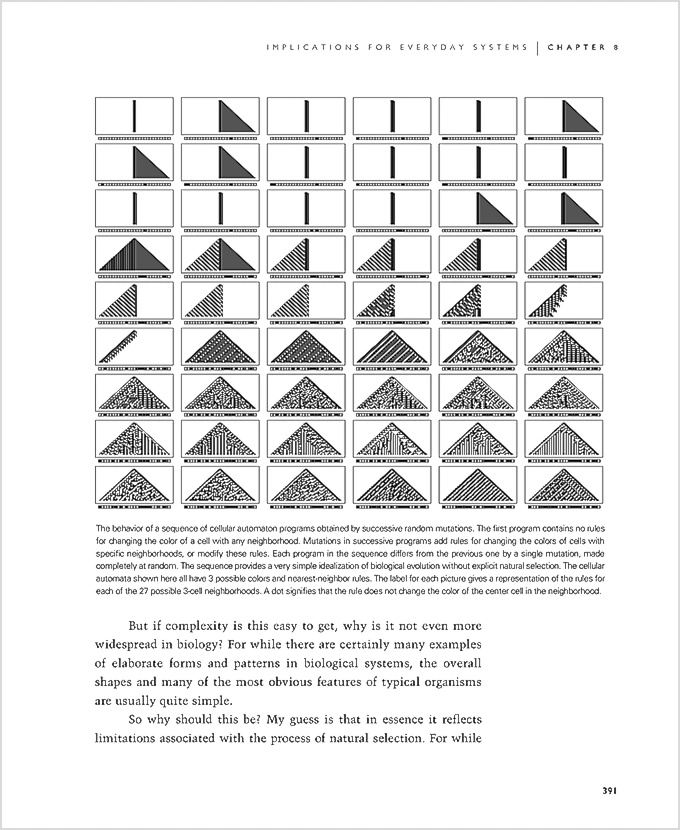
This was not adaptive; it followed a random straight line through rule space. My focus, there and elsewhere in the book, was what systems naturally do rather than what they can be constructed or evolved to do. I did give constructions for particular tasks such as generating primes. In “Intelligence in the Universe,” I also explored finding $k=3,r=1$ rules that double their input, partly to illustrate the difficulty of recognizing purposeful construction versus natural behavior:

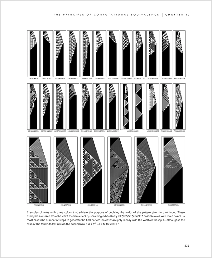
Years passed. Summer School projects occasionally studied rule spaces and adaptation. I retained an interest in biological foundations, gathered information, and gave talks. By the mid-2010s, practical Wolfram Language work had also brought me up to date with modern machine learning, although I had not fully internalized the connection. Around then, Greg Chaitin told me about trying to prove Darwin, as he put it, with computational ideas drawn from his work on mathematical foundations.

Our Physics Project arrived in 2020 with a formalism built around multiway graphs and related concepts. I soon realized that multicomputation, as I called it, was relevant far beyond fundamental physics. By 2021 I was trying to classify its possible applications:

[Image unavailable: the source image is missing.]

The first I pursued seriously was metamathematics, leading to a book in 2022. Later that year, I completed a project fifty years in the making on the second law of thermodynamics, inspired by the Physics Project. It also advanced my thinking about biological systems’ fundamental properties, though not their adaptive evolution.

Then ChatGPT appeared. Alongside technical work involving it, I considered its science, particularly why it works. Part seemed connected to unrecognized regularities in human language. Another part reflected an emerging meta-discovery: train a machine-learning system hard enough and it seems capable of learning almost anything.

Why? Initially I thought high dimensionality made the result obvious, but quickly realized there was much more to it. To explore the boundaries, a few months ago I wrote about whether AI can solve scientific problems:

[Image unavailable: the source image is missing.]

I discussed possible scientific objectives, such as prediction and narrative explanation. Deep in the article, a section on exploring spaces of systems asked questions like whether a system can be found that does X, and whether neural networks can find such systems before an otherwise enormous exhaustive search would. As an aside, I thought comparison with non-neural adaptive evolution might be interesting.

Recalling Chaitin’s connection between the halting problem and evolution, I wondered whether adaptively evolving automaton rules could find patterns with specified finite lifetimes. I imagined a classic machine-learning problem minimizing a loss function.

Just after 1 a.m. on February 22, I wrote three lines of Wolfram Language and tried the experiment:

[Image unavailable: the source image is missing.]

It worked. I found automaton rules producing patterns with lifetime exactly 50:

[Image unavailable: the source image is missing.]

The experiment had indeed found rules that lived exactly 50 steps:

[Image unavailable: the source image is missing.]

In retrospect, I was fortunate. The experiment was so simple, at least in the Wolfram Language, that I tried it despite not expecting success. My first parameter choices—$k=4$, lifetime 50, and so on—also happened to work directly.

In principle, I could have performed the same experiment forty years ago, though less conveniently without the Wolfram Language. My computers were already powerful enough to obtain these results. Without modern machine learning’s example, however, I probably would not have tried, and would certainly have given up readily. I am somewhat embarrassed to have assumed for so long that adaptive evolution lay beyond straightforward experiments. Still, I am glad to illuminate another long-standing mystery. More of the foundations of biology and machine learning may finally be within reach.